Mazda 3 Price Data - Modelling

Modelling car price data with linear regression and regression trees to understand what influences car price depreciation.

CarPrice

Mazda 3

Author

John Bates

Published

May 3, 2023

Given the cleaned dataset that we created in the companion notebook Mazda 3 Price Data - Preparation we now want to attempt to obtain some numerical estimates of how different variables affect the monthly car price depreciation. As in the previous notebook we will be using the tidyverse packages.

We start by reading in the cars tibble that we created and saved.

library(tidyverse)
cars <- readRDS("../01.preparation/mazda3.rds")

We restrict its content to used “Used” cars. And we restrict its content to cars for which we have a value for depreciation_per_month.

cars <- cars |>
  filter(new_used == "Used") |>
  filter(!is.na(depreciation_per_month))

We ended the visualisation notebook with a table of monthly median depreciation values for each combination of variant and engine.

These are ordered in ascending order of the median depreciation per month.

cars |>
  select(depreciation_per_month, variant, engine) |>
  group_by(variant, engine) |>
  summarise(n=n(), median_dpm = median(depreciation_per_month)) |>
  arrange(median_dpm) |>
  knitr::kable(digits=0)

variant	engine	n	median_dpm
SE-L	e-Skyactiv G	41	161
SE-L Lux	e-Skyactiv G	50	187
Sport Lux	e-Skyactiv G	109	194
GT Sport	e-Skyactiv G	50	207
SE-L Lux	e-Skyactiv X	5	213
GT Sport Tech	e-Skyactiv G	39	223
Sport Lux	e-Skyactiv X	26	229
GT Sport	e-Skyactiv X	27	233
GT Sport Tech	e-Skyactiv X	15	249

Figure 1: Summarising by group median.

The difference in depreciation between the SE-L Lux with the e-Skyactiv G engine and the top of the range GT Sport Tech with the e-Skyactiv X engine is about £88 per month.

One method available to us is to perform a linear regression of our independent variables (variant, engine, age_in_months and miles_per_month) on our dependent variable (depreciation_per_month).

There are several assumptions made when using linear regression:

The independent variables are truly independent of each other: This is a reasonable assumption here, especially after we converted depreciation to depreciation_per_month and miles to miles_per_month thereby removing a dependency on age_in_months.
There are no outliers: We will ensure that below.
The variables are normally distributed: This one is a little more tricky. Some are, some not so much.
There is a linear relationship between the independent variables and the dependent variable: An assumption that we will make based on the scatter-plots of the previous notebook.

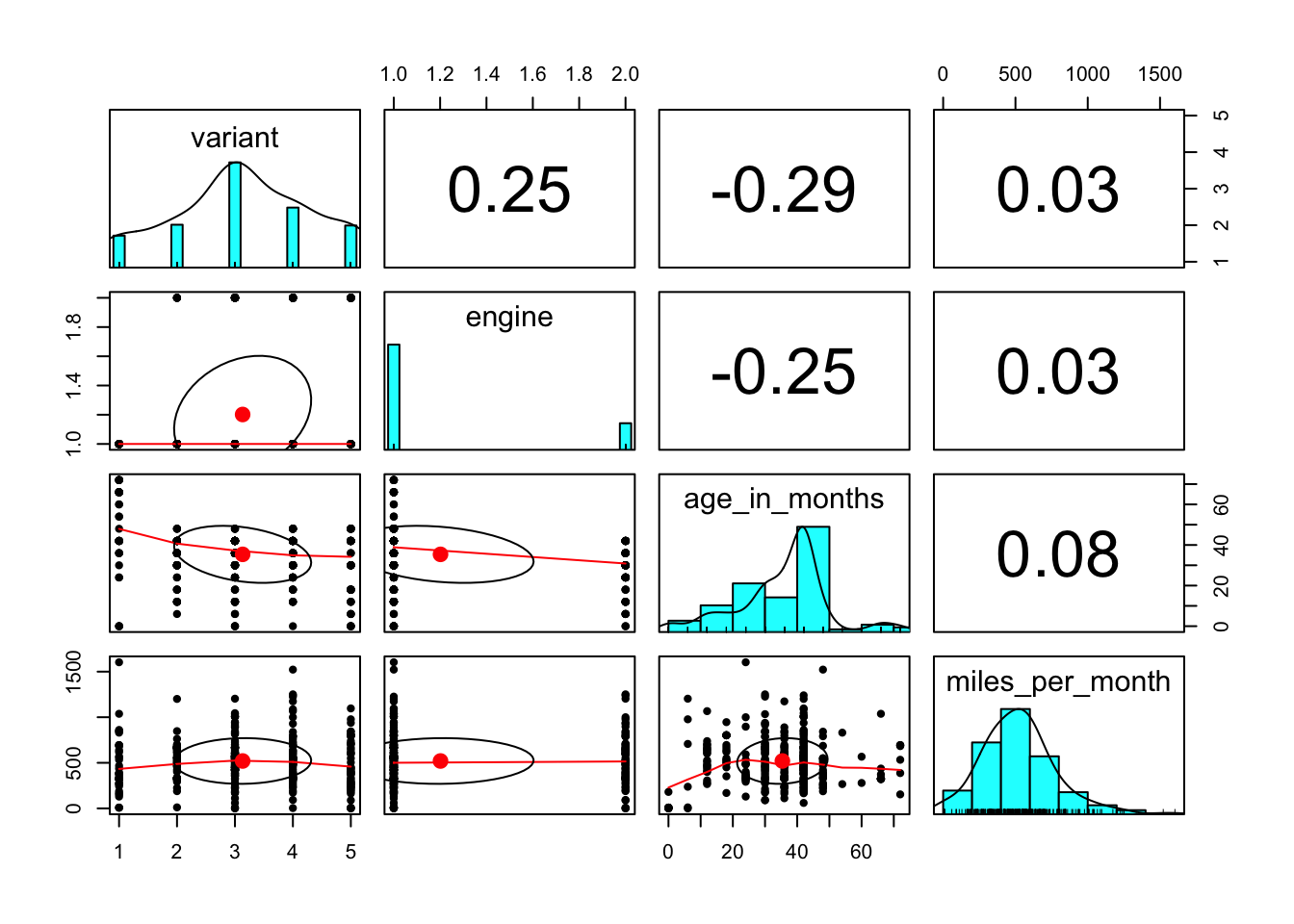
A pairs.panels plot from the psych library confirms that the correlations between the independent variables are low.

library("psych")
pairs.panels(
  cars[c( "variant", "engine","age_in_months", "miles_per_month")],
  cor=T
)

We should also consider removing outliers from our analysis. The outliers are the observations that lie beyond the extremes of the whiskers in a box and whiskers plot. That is, those observations that are more than 1.5 times the interquartile range above or below the 75% and 25% quartiles.

We can see the outliers on the boxplot.

ggplot(
    data = cars,
    mapping = aes(x = depreciation_per_month)
) + geom_boxplot()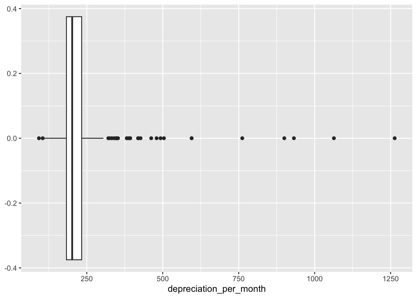

These can be captured and removed by calculating the interquartile range and the 25% and 75% quantiles.

iqr <- IQR(cars$depreciation_per_month)

q25 <- quantile(cars$depreciation_per_month, 0.25)
q75 <- quantile(cars$depreciation_per_month, 0.75)
lower <- q25 - 1.5*iqr
upper <- q75 + 1.5*iqr

outliers <- cars |>
  filter(
      depreciation_per_month > upper
    | depreciation_per_month < lower
  )

We can examine the outliers by variant and engine and then calculate their median depreciation_per_month (dpm), depreciation (d) and age_in_months (a).

outliers |>
  select(
    depreciation_per_month, variant, engine,
    depreciation, age_in_months
  ) |>
  group_by(variant, engine) |>
  summarise(n=n(),
    dpm = median(depreciation_per_month, na.rm=T),
    d=median(depreciation, na.rm=T),
    a=median(age_in_months, na.rm=T)
  ) |>
  arrange(dpm) |>
  knitr::kable(digits=0)

variant	engine	n	dpm	d	a
GT Sport	e-Skyactiv X	1	321	10585	30
SE-L Lux	e-Skyactiv G	1	326	4890	12
GT Sport Tech	e-Skyactiv G	14	350	6782	15
GT Sport	e-Skyactiv G	5	393	5885	12
GT Sport Tech	e-Skyactiv X	2	446	4015	6
Sport Lux	e-Skyactiv X	6	486	4021	9
SE-L	e-Skyactiv G	4	595	2035	0

We notice that the outliers look to be mainly from the very expensive combinations of variant and engine and so it may really be that they were highly depreciated vehicles. We could choose to leave these outliers in for the analysis and treat them as valid observations. But given that they are quite small in number and we will remove them.

cars <- cars |>
  filter(
      depreciation_per_month < upper
    & depreciation_per_month > lower
  )

Linear Regression

To estimate the numeric effect of each of our independent variables on the value of the dependent depreciation_per_month variable we can perform a linear regression on the data.

A linear regression will fit a straight line through the data of the form:

\[ depreciation\_per\_month = \alpha + \beta_1 * variant + \beta_2 * engine ... \]

We will be interested in the value of \(\alpha\), and the accompanying \(\beta\) values. The constant value \(\alpha\) will give us the base monthly depreciation and the the \(\beta\)s will give us the amount by which the predicted monthly depreciation will be increased (or decreased) when a vehicle has the associated variant, or engine size. Or in the case of the continuous independent variables, how much the predicted monthly depreciation will increase with each month of age or mile of travel of the vehicle.

To handle the independent variables that are factors, the model will employ dummy coding to convert each value of the factor into a numeric variable that takes on the value zero or one according as the observation takes on that value of the factor. When performing this conversion the first level of the factor is left out as it represents the situation when all of the other dummy coded factor values for that factor take on the value zero. This will be a little clearer when we look at the results of the regression.

model.lm <- lm(
  depreciation_per_month ~
    variant+engine+age_in_months+miles_per_month,
  data=cars
)
summary(model.lm)


Call:
lm(formula = depreciation_per_month ~ variant + engine + age_in_months + 
    miles_per_month, data = cars)

Residuals:
    Min      1Q  Median      3Q     Max 
-81.155 -11.602  -0.778  10.409 126.978 

Coefficients:
                       Estimate Std. Error t value Pr(>|t|)    
(Intercept)          214.894125   7.507069  28.626  < 2e-16 ***
variantSE-L Lux       -2.849454   5.030114  -0.566    0.571    
variantSport Lux       4.247137   4.369210   0.972    0.332    
variantGT Sport       19.093102   4.731430   4.035 6.82e-05 ***
variantGT Sport Tech  30.810686   5.099644   6.042 4.22e-09 ***
enginee-Skyactiv X    17.621812   3.129154   5.631 3.90e-08 ***
age_in_months         -1.565584   0.115622 -13.541  < 2e-16 ***
miles_per_month        0.069169   0.004908  14.094  < 2e-16 ***
---
Signif. codes:  0 '***' 0.001 '**' 0.01 '*' 0.05 '.' 0.1 ' ' 1

Residual standard error: 20.51 on 321 degrees of freedom
Multiple R-squared:  0.6885,    Adjusted R-squared:  0.6817 
F-statistic: 101.4 on 7 and 321 DF,  p-value: < 2.2e-16

The residuals in the output are an indication of how well (or badly) our model fits the observed values of depreciation_per_month. The first thing to notice is that the maximum and minimum values of the residuals are £126 and -£81 respectively. These are the worst cases. The 50% of observations that fall between the 1Q and 3Q values have residuals that range between -£11 and £11. That seems like a very comfortable range.

Before examining the fitted values we need to look at the goodness of fit. The Adjusted R-squared value of 0.6817 is good. This value gives us an indication of how well our model explains the variation in monthly depreciation - in this case approximately 68%.

We also see that the three stars against each of the independent variables (except for the SE-L Lux and the Sport Lux variants) tell us that it is extremely unlikely that they do not influence the value of our modelled dependent variable, depreciation_per_month.

The model doesn’t consider the SE-L Lux and Sport Lux variants to influence the depreciation_per_month in a significant way.

We can plot the residuals against the fitted values of the model:

predicted <- predict(model.lm)
residuals <- residuals(model.lm)
ggplot(
    data = cars,
    aes(x = predicted, y = residuals)
) + geom_point()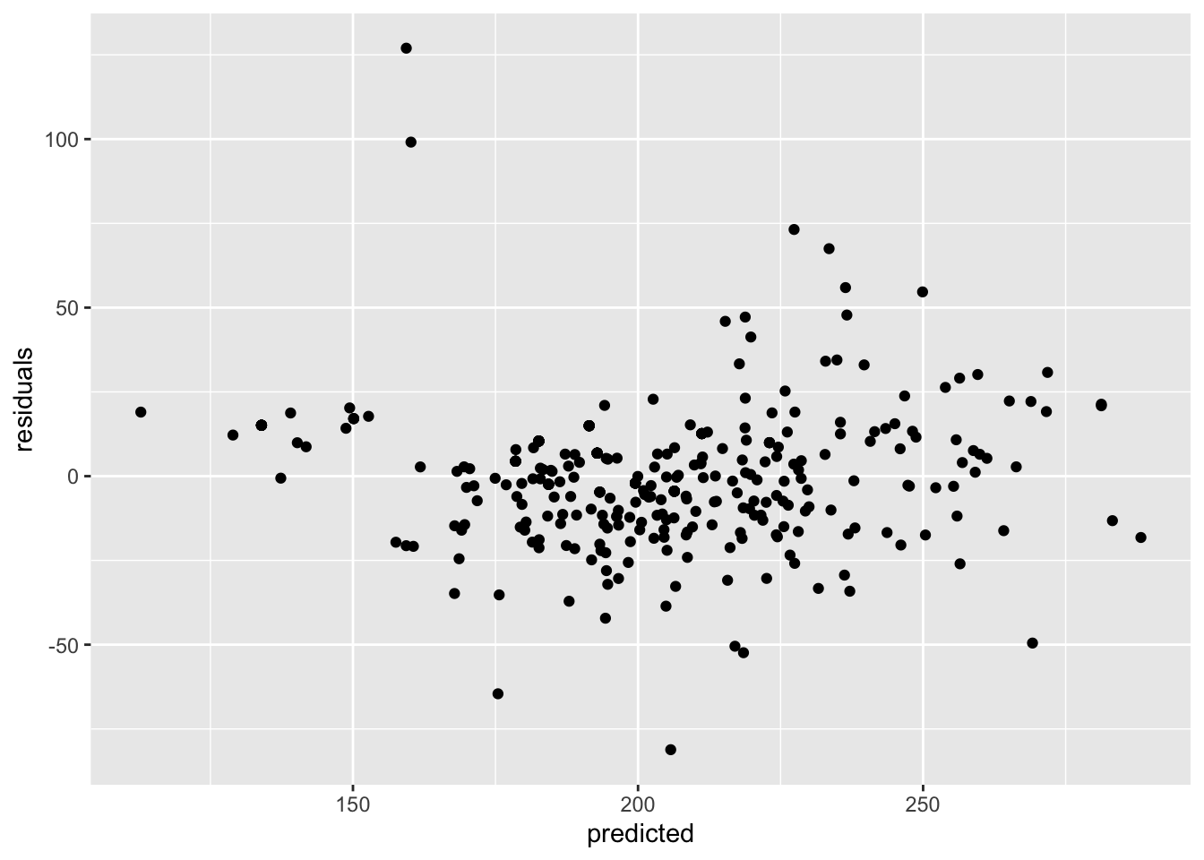

This seems like a reasonable spread, perhaps slightly wider towards the higher end of the predicted values but good enough. Given that we are happy with the fit of the model we can now look at the values of the various fitted coefficients.

Before we can do that though we need to understand how the non-numeric (nominal) dependent variables in our model are handled by the regression. We can see that:

For our 5 level variant variable the model contains 4 parameters: variantSE-L Lux, variantSport Lux, variantGT Sport, variantGT Sport Tech.
For our 2 level engine variable the model contains a single parameter: enginee-Skyactiv X.
For our numeric age_in_months variable the model contains a single parameter: age_in_months.
For our numeric miles_per_month variable the model contains a single parameter: miles_per_month.

The key thing to note is that each non-numeric variable (a factor in our dataset) is represented in the model by (n-1) parameters where n is the number of levels of the factor that represents the nominal variable. The regression ensures that the effect of the first of the factor levels is incorporated into the value of the estimated intercept. To see the effect of having one of the other factor levels in an observation we need to add its associated coefficient to the value of the intercept.

For example, to represent the engine factor our model has a parameter, enginee-Skyactiv X, with a coefficient of (roughly) 18. This tells us that, in general, a vehicle with the e-Skyactiv X engine will depreciate at £18 per month more than a vehicle with the e-Skyactiv G. If we plug the estimated intercept value and the rounded coefficients for the various model parameters into our model equation it looks like this:

  depreciation_per_month = 215
    + 19 * variantGT Sport
    + 30 * variantGT Sport Tech
    + 18 * enginee-Skyactiv X
    - 1.56 * age_in_months
    + 0.07 * miles_per_month

We have omitted the SE-L Lux and Sport Lux parameters from this model because the regression analysis determined that they have an insignificant effect on the monthly depreciation.

The intercept value of £215 can be considered to be the estimated monthly depreciation of a vehicle with variant=SE-L (or SE-L Lux or Sport Lux), engine=e-Skyactiv G, age_in_months=0 and miles_per_month=0.

Were we to replace our variant SE-L with a variant of GT Sport then we should expect our monthly depreciation to increase by £19. If we then further opted for the e-Skyactiv X engine we could add another £18 onto the estimated monthly depreciation.

Similarly for the numeric parameters, if we were to consider the same specification at 12 months old we would subtract 12 * £1.56 = £19 from the estimated monthly depreciation. And 1,000 mile per month of travel would add £70 onto the estimated monthly depreciation.

So the regression gives us a very understandable explanation of how much each of the independent variables affects the value of the monthly depreciation.

Regression Trees

An alternative to using linear regression to model our data is to use regression trees. A regression tree model is built by splitting the set of observations into two partitions in such a way as to maximise the reduction in variation between the observations that lie within each partition. This requires both a choice of feature to split on and then a value with which to partition the data on that feature.

For example, if the miles_per_month feature is chosen as the one that can maximise the reduction in variation, it might then be determined to partition the data into two sets: one whose miles_per_month value was >1000 and one whose miles_per_month value was <= 1000.

This gives us two nodes of a tree. Then the procedure is repeated on the data in each node, giving us four nodes, and so on until there is no significant reduction to be obtained by splitting further.

Once the tree has been constructed by repeating the above process we have:

A set of rules that result in a path to each of the leaf nodes.
A set of homogeneous data in each node from which a mean value of the dependent variable depreciation_per_month can be determined.

For a new observation we can follow the set of rules until we arrive at a leaf node and then we can use the mean value of monthly depreciation of observations in that node as our estimate of the monthly depreciation of the new observation.

To build a regression tree we use the “rpart” package and its associated plotting package.

library(rpart)
library(rpart.plot)

We will build a regression tree model using the same variables that we used for the linear regression model.

model.rt <- rpart(
  depreciation_per_month ~
    variant+engine+age_in_months+miles_per_month,
  data = cars
)

A good visual representation of the regression tree can be obtains by using rpart.plot.

rpart.plot(model.rt)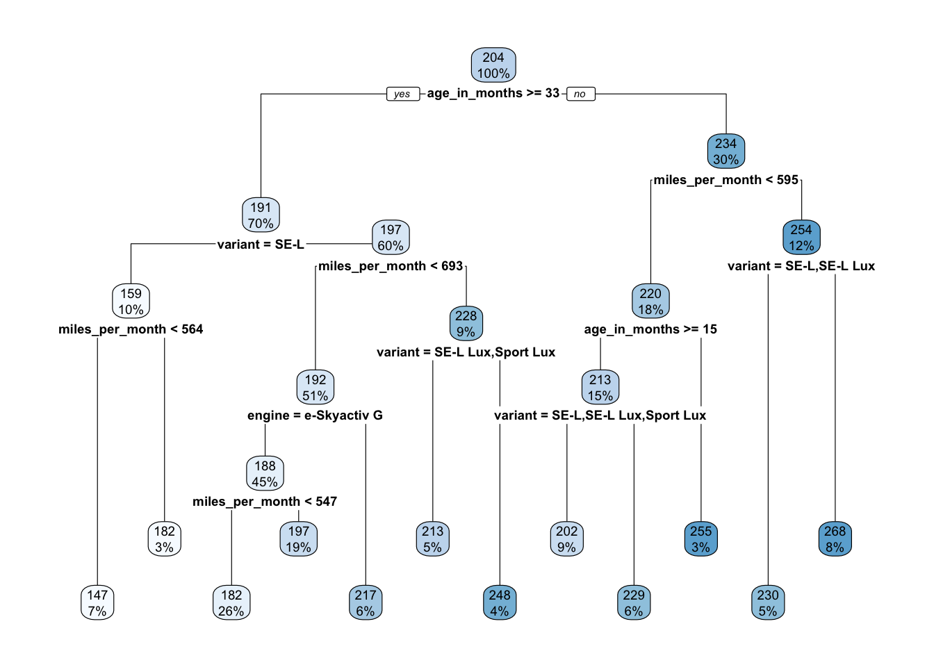

Figure 2: Summarising by regression tree leaf node mean.

We can see that the first variable that was split was age_in_months and that the resulting tree has five levels and terminates in 12 leaf nodes. The values within each node are the mean depreciation_per_month of the observations that fall into that node and the percentage of the observations that reach that point.

Because age_in_months was used first in the tree it is the single most important predictor of the monthly depreciation of a vehicle. The regression model divides the observations on age_in_months >= 33, placing all observations for which this is true in the node on the left-hand-side of the split and all other observations in the node on the right-hand-side.

We can repeat this process right the way down the tree. If we consider the observations for which age_in_months is not greater than 33 (i.e. relatively new vehicles) then the next best predictor of monthly depreciation is miles_per_month. This node tells us that for the higher ‘miles_per_month’ vehicles the next best predictor is ‘variant’ and the cheapest variants (SE-L, SE-L Lux) have an estimated monthly depreciation of £230 and the others an estimated monthly depreciation of £268.

We can get a feel for how good our model is by calculating the mean absolute error.

MAE <- function(actual, predicted) { mean(abs(actual - predicted))}

Normally we would have divided our observations up into a training set and a testing set to perform this operation but here we will use mean absolute error to get a feel for how closely this model can predict our observed monthly depreciation.

predicted <- predict(model.rt, cars)
actual <- cars$depreciation_per_month

print(MAE(actual, predicted))

[1] 14.05005

So, on average, our model predicts the value of the monthly depreciation to within £14 of the observed depreciation. We could think of that as a measure of what we have lost by summarising the data into a structured and explainable model.

Let us look at what we would have obtained had we trained our model on a proportion of the data and then used the remaining observations to test its predictive accuracy.

We use set.seed to ensure that our results are reproducible. We take a random selection of 90% of our observations for the training set and use the remaining 10% to test the resulting model.

set.seed(15151)
n <- (cars |> count())[[1]]
cars_rand <- cars[order(runif(n)),]
split <- round(n*0.9, 0)

cars_train <- cars_rand[1:split, ]
cars_test <- cars_rand[(split+1):n, ]

model.rt.train <- rpart(
  depreciation_per_month ~ variant+engine+age_in_months+miles_per_month,
  data = cars_train
)

We can plot the decision tree of the training model as we did for the model we obtained from the full set of data.

rpart.plot(model.rt.train)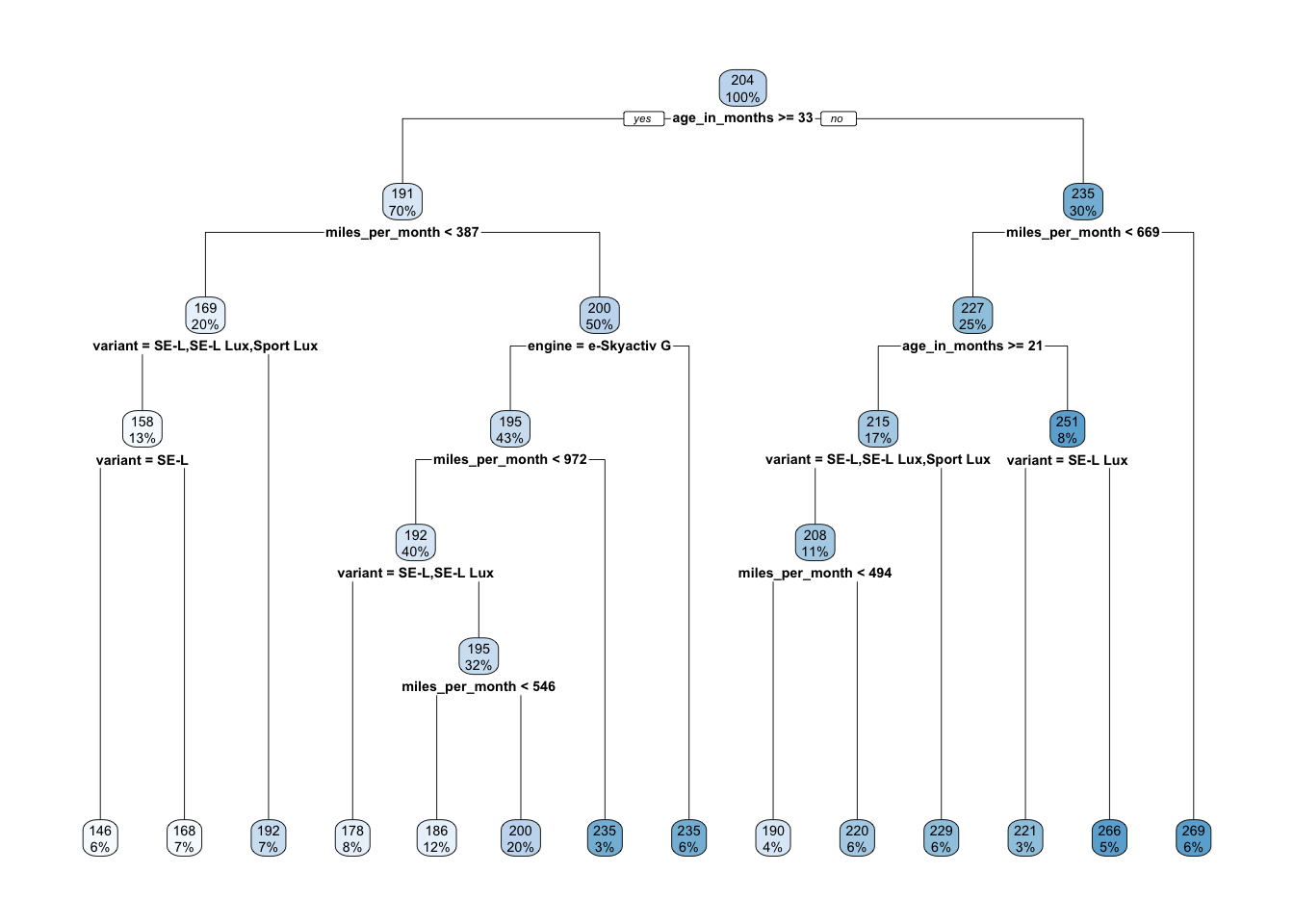

Perhaps unsurprisingly, but somewhat reassuringly, the tree is similar to the previous one. The choice of variable to split on is initially the same, but after that the choice of variable is different. We have a similar number of leaf nodes: 12 vs 14, and the range of ‘depreciation_per_month’ values in the leaf nodes varies from 147 to 268 in one case and from 146 to 269 in the other case.

predicted <- predict(model.rt.train, cars_test)
actual <- cars_test$depreciation_per_month

print(MAE(actual, predicted))

[1] 13.54872

The mean absolute error is roughly the same as the value that we obtained using the data that the model was trained on. This seems like a very small value for error in monthly depreciation, which suggests that our model is a good one.

We have seen how a regression tree can provide an alternative mechanism for understanding what drives monthly depreciation in our car dataset.

Linear Regression vs Regression Tree

We can compare the linear regression and the regression tree by training a new linear regression model on our training set and then calculating the mean absolute error of its predictions using the test data.

model.lm.train <- lm(
  depreciation_per_month ~ variant+engine+age_in_months+miles_per_month,
  data=cars_train
)

summary(model.lm.train)


Call:
lm(formula = depreciation_per_month ~ variant + engine + age_in_months + 
    miles_per_month, data = cars_train)

Residuals:
    Min      1Q  Median      3Q     Max 
-81.127 -10.965  -1.289  11.645  99.596 

Coefficients:
                       Estimate Std. Error t value Pr(>|t|)    
(Intercept)          215.438461   7.496604  28.738  < 2e-16 ***
variantSE-L Lux       -6.485232   5.129025  -1.264 0.207102    
variantSport Lux       3.082882   4.397253   0.701 0.483811    
variantGT Sport       18.638074   4.797640   3.885 0.000127 ***
variantGT Sport Tech  30.581669   5.209184   5.871 1.19e-08 ***
enginee-Skyactiv X    17.620848   3.148847   5.596 5.11e-08 ***
age_in_months         -1.622082   0.116082 -13.974  < 2e-16 ***
miles_per_month        0.073328   0.005108  14.356  < 2e-16 ***
---
Signif. codes:  0 '***' 0.001 '**' 0.01 '*' 0.05 '.' 0.1 ' ' 1

Residual standard error: 19.81 on 288 degrees of freedom
Multiple R-squared:  0.7165,    Adjusted R-squared:  0.7096 
F-statistic:   104 on 7 and 288 DF,  p-value: < 2.2e-16

A look at the model parameters confirms that it has hardly changed from the model that was fitted on the full set of data.

predicted.rt <- predict(model.rt.train, cars_test)
predicted.lm <- predict(model.lm.train, cars_test)

print(str_glue(
  "MAE of regression tree:",
  round(MAE(actual, predicted.rt),2))
)

MAE of regression tree:13.55

print(str_glue(
  "MAE of linear regression:",
  round(MAE(actual, predicted.lm),2))
)

MAE of linear regression:14.52

The errors are almost identical, with the regression tree slightly out performing the linear regression.

We now have two useful models of monthly depreciation that can be used to examine what drives depreciation on used Mazda 3 cars in the UK.

In the next notebook we will look at a mechanism for creating a simple two-dimensional table to display aggregated car price data.

Next: Mazda 3 Price Data - Tabulation

Comparing Predictions

We can compare the predictions from the table given at the beginning of this notebook (Figure 1), with the predictions taken from our regression tree (Figure 2), with the predictions of our linear regression. In the last two cases we will use the models built with the full data set, model.lm and model.rt.

To do this we need to build a tibble containing a set of vehicle specifications for which we would like to predict the depreciation per month. We are interested in how each method predicts depreciation per month for vehicles between 6 and 36 months old, and for each combination of variant and engine. That gives us a total of 6 x 5 x 2 = 60 combinations but we need to remove those six invalid combinations that pair the “SE-L” variant with the “e-Skyactiv X”. After removing the invalid combinations we are left with 54 different combinations. We will assume that our vehicles will drive a modest 400 miles per month.

library(dplyr)
variants <- cars |> distinct(variant)
engines <- cars |> distinct(engine) 
age_in_months <- tibble(age_in_months = c(6, 12, 18, 24, 30, 36)) 
car.samples <- variants |>
  cross_join(engines) |>
  cross_join(age_in_months) |>
  mutate(miles_per_month = 400) |>
  filter(!(variant == "SE-L" & engine == "e-Skyactiv X"))

We can start with the linear regression and the regression tree models and use their predict function to generate a predicted monthly depreciation for each of our 54 synthetic observations.

dpm.lm <- predict(model.lm, car.samples)
dpm.rt <- predict(model.rt, car.samples)

summary(dpm.lm)

   Min. 1st Qu.  Median    Mean 3rd Qu.    Max. 
  183.4   212.2   228.6   228.9   244.9   281.6

summary(dpm.rt)

   Min. 1st Qu.  Median    Mean 3rd Qu.    Max. 
  147.5   202.1   228.8   224.2   254.8   254.8

Although the minimum and maximum depreciation_per_month values for the regression tree model are about £30 less than those for the linear regression, the interquartile range is almost identical and so is the median value.

To compare these with the predictions that we might make using the table shown in Figure 1 is slightly more complicated. These predictions will have to ignore both age_in_months and miles_per_month because our table does not contain that information. Instead, they will use the median depreciation_per_month for the combination of variant and engine. We can see from the table that each valid combination of variant and engine is represented.

We will create a lookup tibble using a grouping of variant and engine, and for each group we will work out the median depreciation_per_month.

lookup <- cars |>
  select(depreciation_per_month, variant, engine) |>
  group_by(variant, engine) |>
  summarise(median_dpm = median(depreciation_per_month))

We can then obtain a prediction from the table for each of our observations by performing a left outer join between the observations tiblle and the lookup tibble.

dpm.tab <- car.samples |>
  left_join(lookup, by = c("variant", "engine")) |>
  select(depreciation_per_month = median_dpm) |>
  pull(depreciation_per_month)

We can now add the three prediction columns into our car.samples tibble and also add an observation number column to allow us to uniquely identify each row.

car.samples <- car.samples |>
  mutate(
    dpm.lm = dpm.lm, dpm.rt = dpm.rt, dpm.tab = dpm.tab,
    obs = row_number()
  )

Ordinarily we might randomise the order of the observations to ensure that no particular significance was given to their order. We would use code like this to perform the randomisation.

# We will not do this here because
# we want to see the pattern of our observations.
set.seed(0)
obs <- sample.int(nrow(car.samples), replace=F)
car.samples$obs = obs

But we will not do that here. Not doing the randomisation allows us to see in the predicted depreciation_per_month the effect of the order of the observations: variant then engine then age_in_months.

library(patchwork)
p1 <- ggplot(data = car.samples, mapping=aes(x = obs, shape=age_in_months)) +
  geom_point(mapping = aes(y = dpm.lm), colour="red") +
  scale_shape_binned(labels = function(x) paste(x, "months")) +
  ggtitle("Linear Regression")
p2 <- ggplot(data = car.samples, mapping=aes(x = obs, shape=age_in_months)) +
  geom_point(mapping = aes(y = dpm.rt), colour="red") +
  scale_shape_binned(labels = function(x) paste(x, "months")) +
  ggtitle("Regression Tree")
p3 <- ggplot(data = car.samples, mapping=aes(x = obs, shape=age_in_months)) +
  geom_point(mapping = aes(y = dpm.tab), colour="red") +
  scale_shape_binned(labels = function(x) paste(x, "months")) +
  ggtitle("Tabulated Median")
p1 + p2 + p3 +
  plot_layout(nrow = 3, ncol = 1, guides = "collect")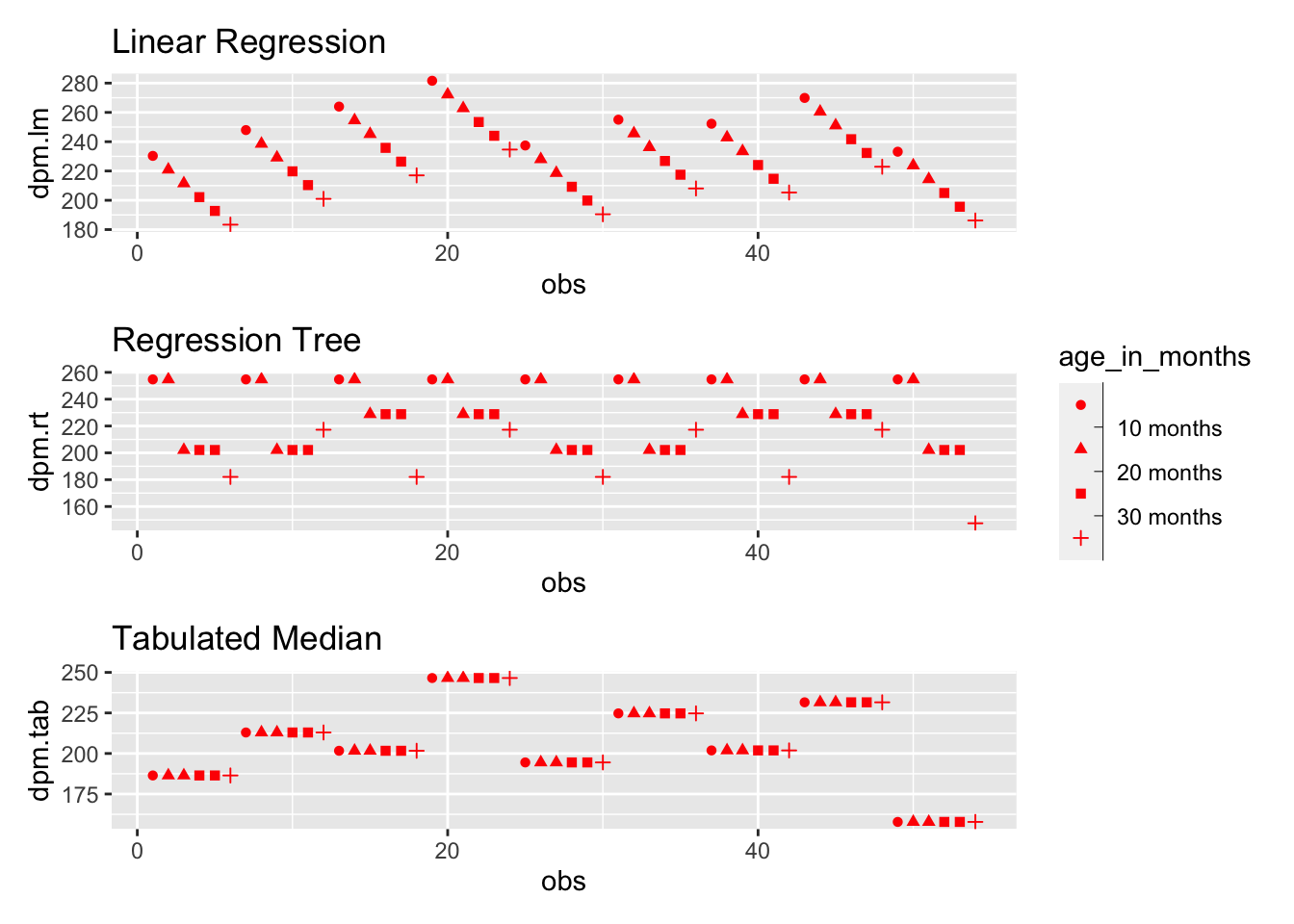

We can clearly see in the linear regression plot the clusters of variant and engine and, within them, the downward sloping decrease in depreciation per month as age_in_months increases.

In the regression tree plot we see clusters of variant and engine in one leaf and then vehicles with the same combination of variant and engine falling into a cluster with lower depreciation_per_month as the age_in_months increases.

For the tablulated median prediction, which does not consider age_in_months, we see a single cluster for each combination of engine and variant - as we would expect.

We recall from our earlier calculation of mean absolute error that the linear regression and the regression tree methods of predicting appeared to be equally as good at reducing error. From the shape of their predicted values shown in the charts above you might think that linear regression would have the edge over regression trees because it appears to smoothly interpolate rather than predict one of a discrete number of bucket values. But perhaps the disadvantage that the linear regression model has is that it has to come up with a linear expression that predicts depreciation_per_month across the complete range of variant, engine and miles_per_month. The regression tree model, is able to first home in on the effect a combination of the model variables has before choosing an appropriate aggregate value for that combination.

If we look at just how much the mean absolute difference is between predictions from these two models for each combination of variant and engine we see that there isn’t much to chose between them.

car.samples |>
  select(variant, engine, dpm.lm, dpm.rt) |>
  group_by(variant, engine) |>
  summarise( mae = MAE(dpm.lm, dpm.rt)) |>
  pivot_wider(names_from=engine, values_from=mae) |>
  knitr::kable(digits=0)

variant	e-Skyactiv G	e-Skyactiv X
SE-L	19	NA
SE-L Lux	13	15
Sport Lux	13	15
GT Sport	10	11
GT Sport Tech	12	23

Figure 3: Mean absolute error difference between linear regression and regression trees.

And if we introduce a breakdown into columns that show age_in_months we, also, see that the difference between the two models appears to have no obvious visual difference between low or high mileage vehicles.

car.samples |>
  select(variant, engine, age_in_months, dpm.lm, dpm.rt) |>
  group_by(variant, engine, age_in_months) |>
  summarise( mae = MAE(dpm.lm, dpm.rt)) |>
  pivot_wider(names_from=age_in_months, values_from=mae) |>
  knitr::kable(digits=0)

variant	engine	6	12	18	24	30	36
SE-L	e-Skyactiv G	22	31	12	3	7	39
SE-L Lux	e-Skyactiv G	24	34	9	0	9	1
SE-L Lux	e-Skyactiv X	7	16	27	18	8	16
Sport Lux	e-Skyactiv G	17	27	16	7	2	8
Sport Lux	e-Skyactiv X	0	9	34	25	15	9
GT Sport	e-Skyactiv G	3	12	5	5	14	23
GT Sport	e-Skyactiv X	15	6	22	13	3	6
GT Sport Tech	e-Skyactiv G	9	0	16	7	2	35
GT Sport Tech	e-Skyactiv X	27	17	34	25	15	17

Figure 4: Mean absolute error difference between linear regression and regression trees additionally broken down by age in months.

So we have two mechanisms, linear regression and regression trees, for predicting the monthly depreciation of a Mazda 3 for a given variant, engine choice and age_in_months given an estimated mileage_per_month with neither model clearly better than the other.

Next: Mazda 3 Price Data - Tabulation