library(tidyverse)
cars <- readRDS("../01.preparation/mazda.rds")Mazda CX-30 Price Data - Visualisation
Examining car price data to understand what influences car price depreciation.
R
CarPrice
Mazda CX-30
Given the cleaned dataset that we created in the companion notebook Mazda 3 Price Data - Preparation we can now start to look more closely at the factors that influence used car depreciation for our chosen model, the Mazda CX-30. As in the previous notebook we will be using the tidyverse packages.
We start by reading in the cars tibble that we created and saved.
For the purposes of understanding depreciation we need to limit our data to used cars. That can be done very simply with the filter function of the tidyverse dplyr package.
cars <- cars |>
  filter(new_used == "Used")
We can see that the data consists of several hundred rows on 14 columns. These represent several hundred observations on 14 variables - each row or observation is of a single vehicle and each observation has a value for each of the 14 variables.
There are some situations in which the value of a variable may be unknown for an observation. In such a case the value is represented with NA which we can think of as meaning missing. In most cases we will reject observations for which we have missing data.
str(cars)tibble [493 × 14] (S3: tbl_df/tbl/data.frame)
$ model : Factor w/ 1 level "Mazda CX-30": 1 1 1 1 1 1 1 1 1 1 ...
$ variant : Factor w/ 5 levels "SE-L","SE-L Lux",..: 5 1 2 5 5 1 5 4 4 5 ...
$ drive : Factor w/ 2 levels "2WD","AWD": 1 1 1 1 1 1 1 1 2 1 ...
$ engine : Factor w/ 2 levels "e-Skyactiv G",..: 2 1 1 2 2 1 2 2 2 2 ...
$ new_used : Factor w/ 2 levels "Used","New": 1 1 1 1 1 1 1 1 1 1 ...
$ miles : num [1:493] 6542 14814 17548 225 33258 ...
$ miles_per_month : num [1:493] 312 494 450 75 853 ...
$ price : num [1:493] 24990 18785 21995 29994 21495 ...
$ price_new : num [1:493] 31815 24645 26145 31815 31815 ...
$ depreciation : num [1:493] 6825 5860 4150 1821 10320 ...
$ depreciation_per_month: num [1:493] 325 195 106 607 265 ...
$ fuel : Factor w/ 1 level "Petrol": 1 1 1 1 1 1 1 1 1 1 ...
$ transmission : Factor w/ 1 level "Manual": 1 1 1 1 1 1 1 1 1 1 ...
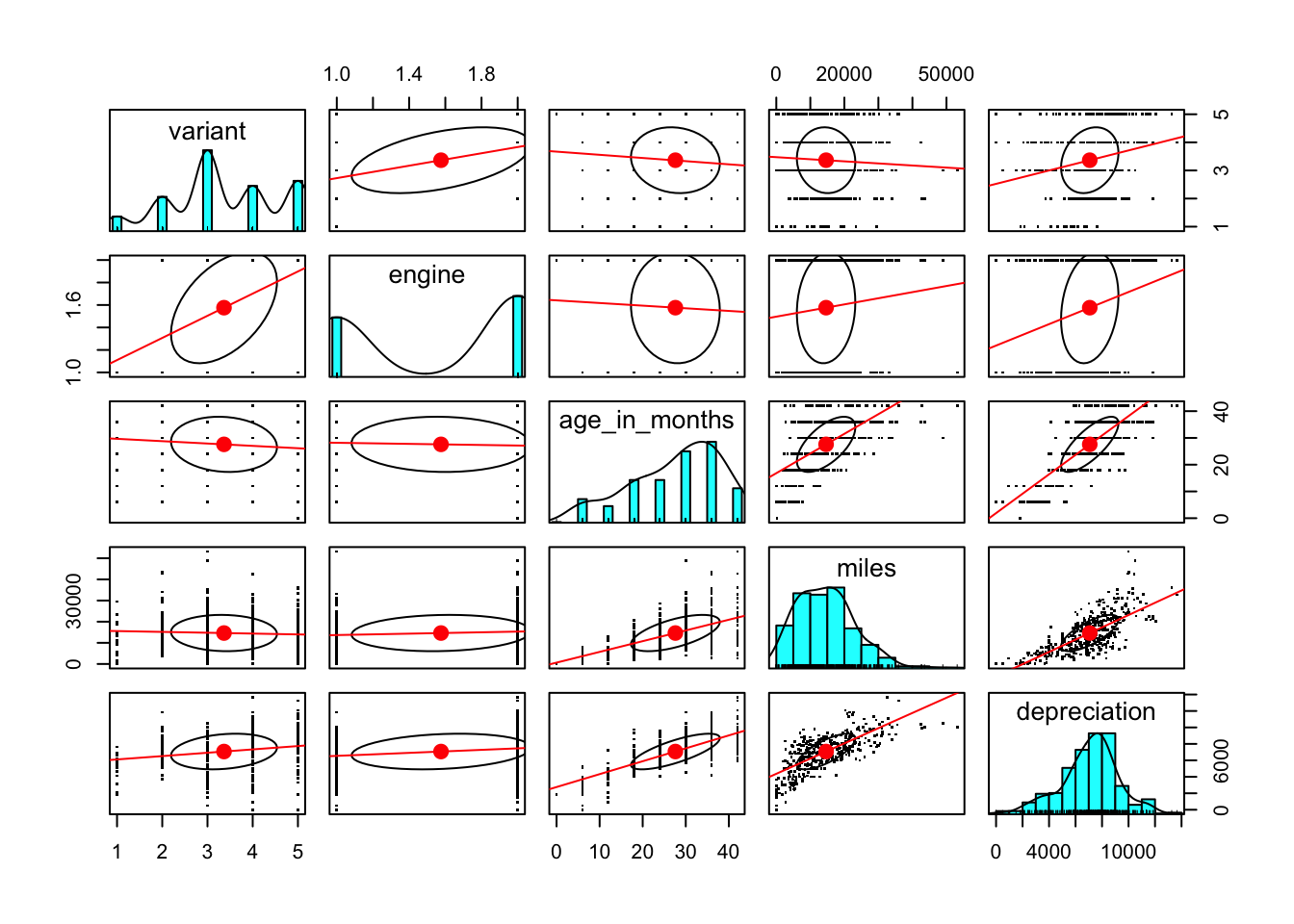
$ age_in_months : num [1:493] 18 24 36 0 36 24 30 6 30 24 ...A good place to start is to look at the relationships between the columns using a pairs plot. This plot uses the pairs.panels plot from the psych package to show, in addition to the normal pairs scatterplots, some information about the correlations between each displayed column.
The diagonal shows a histogram of the values of each variable. This gives us a visual indication of the distribution of values of that variable.
Above and below the diagonal are plots of each pairwise combinations of variable. The plots are overlaid by a linear regression line and a correlation ellipse. These indicate the general tendency of high values of one variable to be associated with high or low values of the other variable. A circular correlation ellipse indicates no such association.
library("psych")
pairs.panels(
  cars[c(
    "variant", "engine", "age_in_months",
    "miles", "depreciation"
  )],
  pch = ".",
  cor=F,
  lm = T,
  )
Note
In addition to the list of variables to plot, the call to pairs.panels has three other parameters: pch, cor and lm.
Because there are so many data points to plot the pch parameter allows us to replace the default plot symbol, which is a bullet character (pch=20), with an alternative. Setting it to “.” is a special case which results in a plot very small rectangle used as the plot symbol.
Setting cor to false prevents the plot from displaying Pearson correlation coefficients. These are often useful but should really only be used when the distribution of the variables being compared is close to a normal distribution.
Setting lm to true gives us a linear regression line for each pair of variables in addition to the correlation ellipse.
The most obvious observation is that depreciation increases with both age of the vehicle and the number of miles that it has been driven. That is not surprising, but it is a reminder that depreciation is not really the variable that we are interested in. A more interesting value to measure would be depreciation over time.
Similarly, a measure of miles, being so highly correlated with age_in_months might be more usefully expressed as miles_per_month. Fortunately, we recognised that when preparing the data and we do have two variables, miles_per_month and depreciation_per_month, which attempt to correct the effect that age has on miles driven and depreciation.
If we we create the pairs plot using miles_per_month in place of miles and depreciation_per_month in place of depreciation we see a different picture.
library("psych")
pairs.panels(
  cars[
    c("variant", "engine", "age_in_months",
      "miles_per_month", "depreciation_per_month")],
    pch = ".",
    cor=F,
    lm = T
  )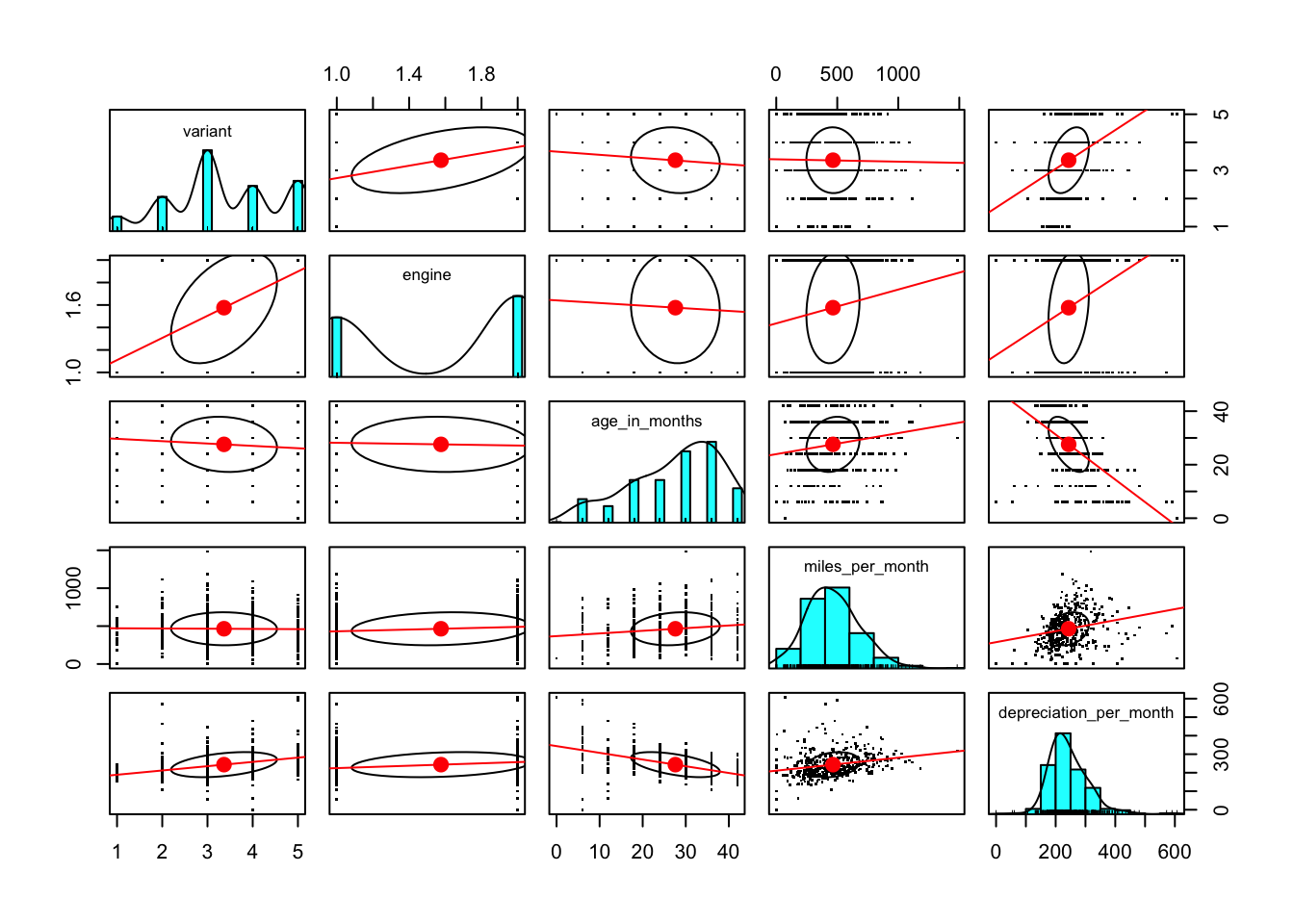
We see that a higher value of age_in_months is associated with a lower value of depreciation_per_month. That feels right, as a vehicle would be expected to lose value more quickly when it was newer. We also see that a higher value of miles_per_month is associated with a higher value of depreciation_per_month. Again, this is something that we might expect to see although it looks to be less highly correlated.
The plot of depreciation_per_month by variant suggests that there might be a high level of association between variant and depreciation_per_month but the fact that variant has only a small number of discrete values and the assumptions about variables being normally distributed mean that we should not put too much weight on the shape of the correlation ellipse for those two variables.
But it might be interesting to view the smoothed distribution of values of depreciation_per_month for each of the variants.
library(ggridges)

cars |> ggplot(
  aes(x = depreciation_per_month, y = variant, fill = variant, color = variant)
) + geom_density_ridges(alpha = 0.5, show.legend = FALSE)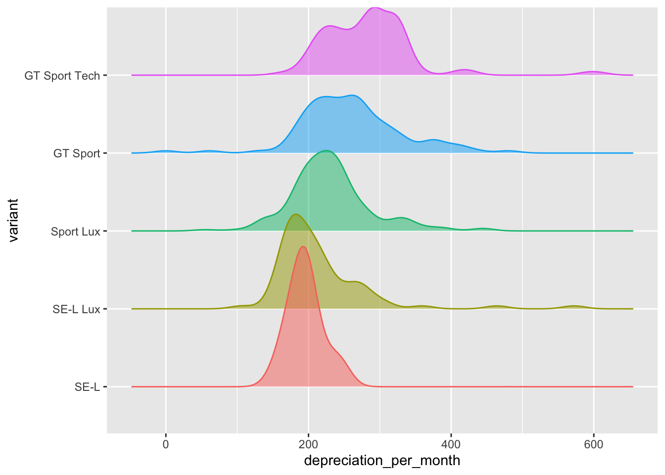
It is noticeable how much narrower the range of depreciation per month is for the cheapest model - the SE-L variant. This is seen even more clearly with a box and whisker plot.
ggplot(
    data = cars,
    mapping = aes(x = depreciation_per_month, y = variant)
) + geom_boxplot(notch = T) 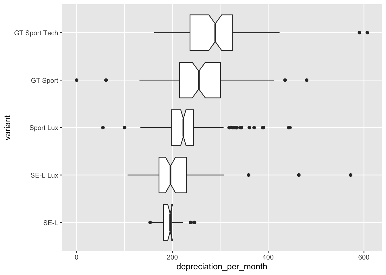
In this plot we have requested a notch on each plot. If the notches on two plots do not overlap then we can assume, with 95% confidence, that the medians are different. So between our variants the median depreciation_per_month is significantly different for all but the SE-L and SE-L Lux variants.
It doesn’t seem too surprising that there would be some vehicles with high levels of depreciation but the low levels are worth examining.
cars |>
  arrange(depreciation_per_month) |>
  select(model, variant, miles, price, price_new,
    dpm = depreciation_per_month) |>
  head(5)
# A tibble: 5 × 6
model variant miles price price_new dpm
<fct> <fct> <dbl> <dbl> <dbl> <dbl>
1 Mazda CX-30 GT Sport 10 31805 30915 0
2 Mazda CX-30 Sport Lux 5 26500 26995 55
3 Mazda CX-30 GT Sport 2705 29994 30915 61.4
4 Mazda CX-30 Sport Lux 25 27500 29005 100.
5 Mazda CX-30 SE-L Lux 17548 21995 26145 106. We can see that these are all low mileage vehicles that are priced close to (or above in one case) our estimate of their new price.
We can introduce the value of the engine variable into our boxplot to see whether that has an impact on monthly depreciation.
ggplot(
    data = cars,
    mapping = aes(x = depreciation_per_month, y = variant, color=engine)
) + geom_boxplot(show.legend = T, notch = T) 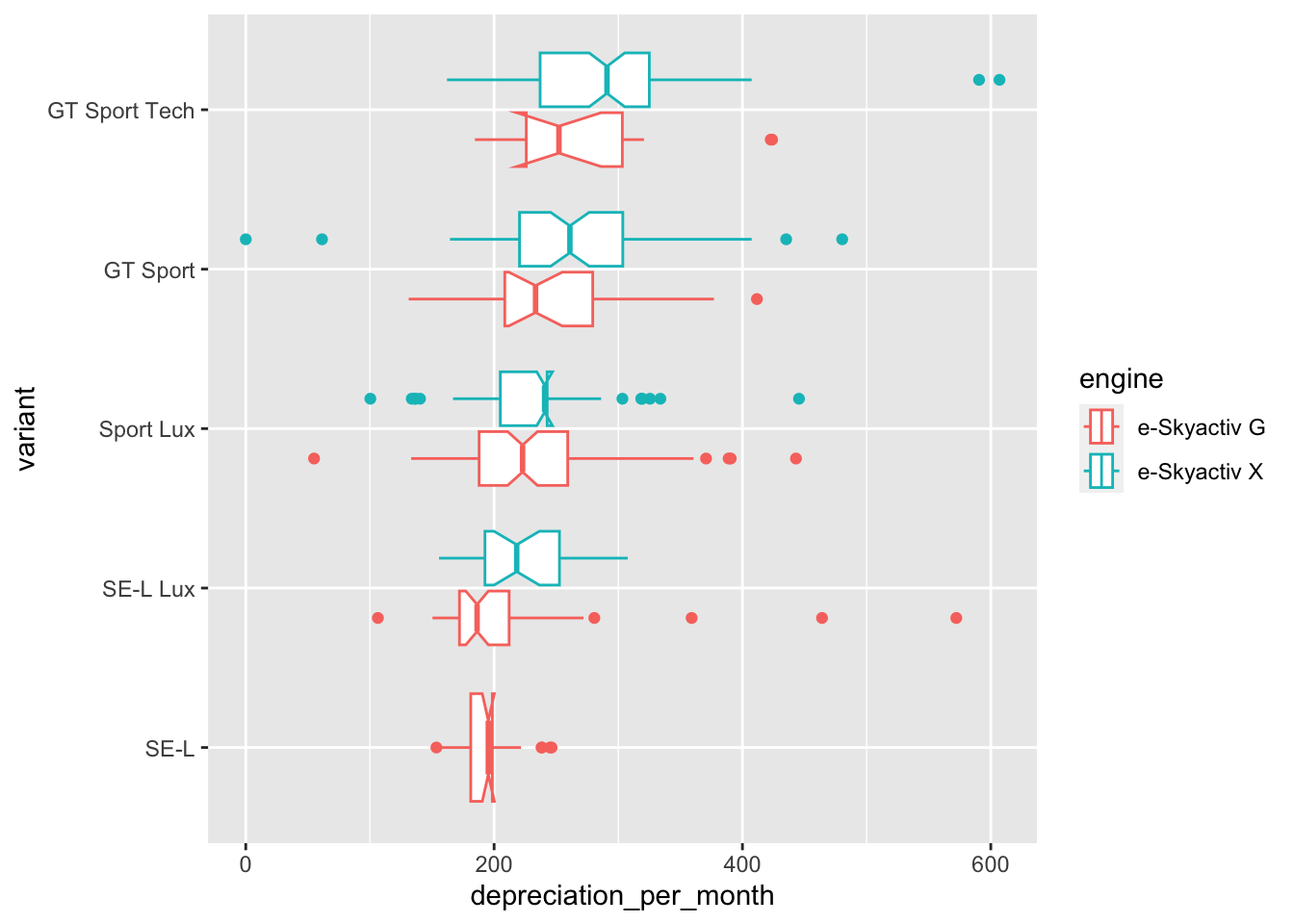
Now the boxplot for each variant has been replace by two boxplots, one for each of the two available engines. The cheapest variant is only available in the e-Skyactiv G engine and so only has the one plot.
For each variant it appears as though the choice of engine also has a significant impact on the median monthly depreciation of the vehicle.
Swapping the Y-axis around and this time diplaying engine in place of variant shows us that even within vehicles with the same engine there is some significant difference in monthly depreciation between the variants.
ggplot(
    data = cars,
    mapping = aes(x = depreciation_per_month, y = engine, color=variant)
) + geom_boxplot(show.legend = T, notch = T) 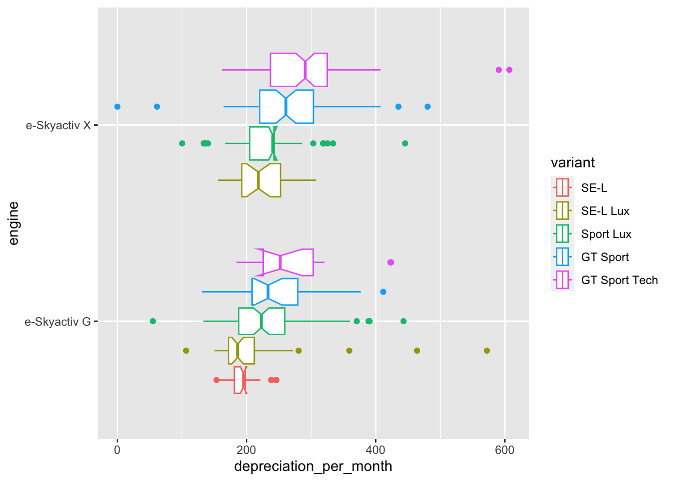
Another observation that becomes clear from the last two plots is that for the cheaper engine, the e-Skyactiv G, there is a slightly smaller monthly depreciation with the SE-L Lux variant when compared with the cheaper SE-L variant.
We can examine the median values of depreciation_per_month by variant in tabular form and this looks to agree nicely with our boxplot above:
cars |>
  select(dpm=depreciation_per_month, variant, engine, drive) |>
  group_by(variant) |>
  summarise(n=n(), median_dpm = median(dpm, na.rm = T)) |>
  arrange(median_dpm) |>
knitr::kable(digits=0)| variant | n | median_dpm |
|---|---|---|
| SE-L | 32 | 195 |
| SE-L Lux | 75 | 196 |
| Sport Lux | 177 | 223 |
| GT Sport | 99 | 255 |
| GT Sport Tech | 110 | 290 |
By engine across all variants and drives:
cars |>
  select(dpm=depreciation_per_month, variant, engine, drive) |>
  group_by(engine) |>
  summarise(n=n(), median_dpm = median(dpm, na.rm = T)) |>
  arrange(median_dpm) |>
knitr::kable(digits=0)| engine | n | median_dpm |
|---|---|---|
| e-Skyactiv G | 209 | 208 |
| e-Skyactiv X | 284 | 244 |
So the effect of the more expensive engine looks to be to increase the monthly depreciation by about £35 across all variants and drives.
By drive across all variants and engines:
cars |>
    select(depreciation_per_month, variant, engine, drive) |>
    group_by(drive) |>
    summarise(n=n(), median_dpm = median(depreciation_per_month, na.rm = T)) |>
    arrange(median_dpm) |>
knitr::kable(digits=0)| drive | n | median_dpm |
|---|---|---|
| 2WD | 468 | 228 |
| AWD | 25 | 305 |
The effect all-wheel-drive increases the monthly depreciation by about £75 across all variants and engines. Or by all combinations of variant, engine and drive.
cars |>
    select(depreciation_per_month, variant, engine, drive) |>
    group_by(variant, engine, drive) |>
    summarise(n=n(), median_dpm = median(depreciation_per_month, na.rm = T)) |>
    arrange(median_dpm) |>
knitr::kable(digits=0)| variant | engine | drive | n | median_dpm |
|---|---|---|---|---|
| SE-L Lux | e-Skyactiv G | 2WD | 48 | 186 |
| SE-L | e-Skyactiv G | 2WD | 32 | 195 |
| SE-L Lux | e-Skyactiv X | 2WD | 27 | 218 |
| Sport Lux | e-Skyactiv G | 2WD | 88 | 223 |
| GT Sport | e-Skyactiv G | 2WD | 27 | 233 |
| Sport Lux | e-Skyactiv X | 2WD | 89 | 241 |
| GT Sport Tech | e-Skyactiv G | 2WD | 14 | 252 |
| GT Sport | e-Skyactiv X | 2WD | 60 | 253 |
| GT Sport Tech | e-Skyactiv X | 2WD | 83 | 285 |
| GT Sport | e-Skyactiv X | AWD | 12 | 304 |
| GT Sport Tech | e-Skyactiv X | AWD | 13 | 306 |
It soon becomes clear that it is difficult to settle on a single method of determining which variables are most explanatory in understanding monthly depreciation. And also, exactly what the numerical effect of the choice of a particular variant, engine or drive might be on monthly depreciation. We have conveniently ignored the effect of the age of the vehicle or the number of miles it has been driven and we know that these are likely to have a big effect.
In the next notebook we will look to model the effect of all of these variables on monthly depreciation.