Mazda 3 Price Data - Visualisation

Examining car price data to understand what influences car price depreciation.

CarPrice

Mazda 3

Author

John Bates

Published

May 2, 2023

Given the cleaned dataset that we created in the companion notebook Mazda 3 Price Data - Preparation we can now start to look more closely at the factors that influence used car depreciation for our chosen model, the Mazda 3.

We start by reading in the cars tibble that we created and saved.

library(tidyverse)
cars <- readRDS("../01.preparation/mazda3.rds")

For the purposes of understanding depreciation we need to limit our data to used cars.

cars <- cars |>
  filter(new_used == "Used")

We can see that the data consists of 362 rows on 14 columns.

str(cars)

tibble [362 × 14] (S3: tbl_df/tbl/data.frame)
 $ model                 : Factor w/ 1 level "Mazda 3": 1 1 1 1 1 1 1 1 1 1 ...
 $ variant               : Factor w/ 5 levels "SE-L","SE-L Lux",..: 5 2 2 5 3 3 4 4 2 4 ...
 $ drive                 : Factor w/ 1 level "2WD": 1 1 1 1 1 1 1 1 1 1 ...
 $ engine                : Factor w/ 2 levels "e-Skyactiv G",..: 1 1 1 1 1 1 1 1 1 2 ...
 $ new_used              : Factor w/ 2 levels "Used","New": 1 1 1 1 1 1 1 1 1 1 ...
 $ miles                 : num [1:362] 16843 12875 7891 28947 25664 ...
 $ miles_per_month       : num [1:362] 802 330 292 643 570 ...
 $ price                 : num [1:362] 21000 17250 19995 18995 16500 ...
 $ price_new             : num [1:362] 28285 24385 24385 28285 25485 ...
 $ depreciation          : num [1:362] 7285 7135 4390 9290 8985 ...
 $ depreciation_per_month: num [1:362] 347 183 163 206 200 ...
 $ fuel                  : Factor w/ 1 level "Petrol": 1 1 1 1 1 1 1 1 1 1 ...
 $ transmission          : Factor w/ 1 level "Manual": 1 1 1 1 1 1 1 1 1 1 ...
 $ age_in_months         : num [1:362] 18 36 24 42 42 42 30 42 12 24 ...

A good place to start is to look at the relationships between the columns using a pairs plot. This plot uses the pairs.panels plot from the psych package to show, in addition to the normal pairs scatterplots, some information about the correlations between each displayed column.

The diagonal shows a histogram of the values of each variable. This gives us a visual indication of the distribution of values of that variable.

Above and below the diagonal are plots of each pairwise combinations of variable. The plots are overlaid by a linear regression line and a correlation ellipse. These indicate the general tendency of high values of one variable to be associated with high or low values of the other variable. A circular correlation ellipse indicates no such association.

library("psych")
pairs.panels(
  cars[c(
    "variant", "engine", "age_in_months",
    "miles", "depreciation"
  )],
  pch = ".",
  cor=F,
  lm = T,
  )

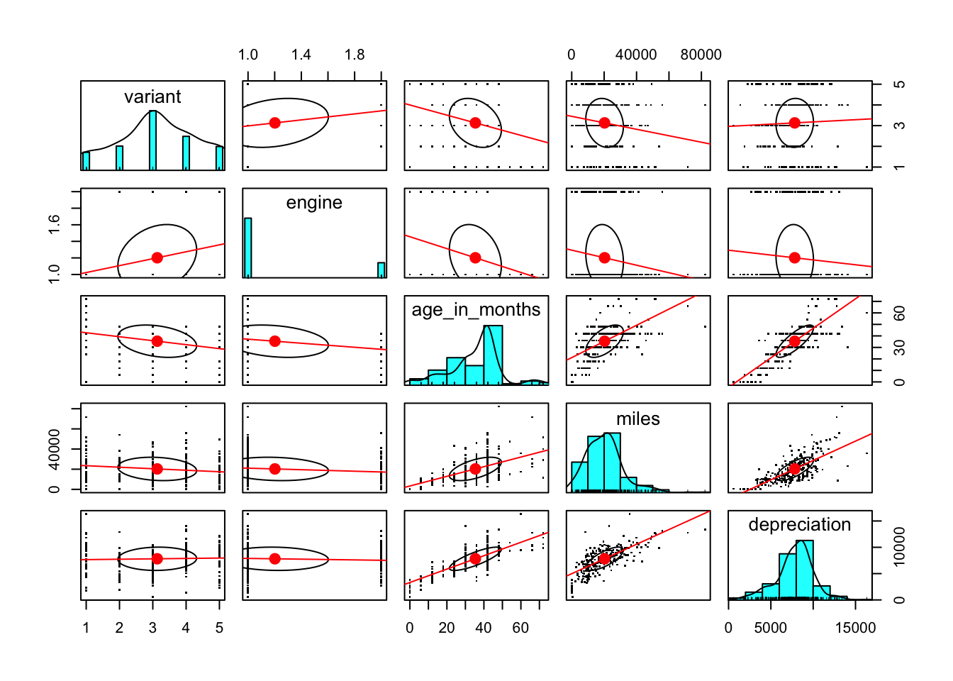
The most obvious observation is that depreciation increases with both age of the vehicle and the number of miles that it has been driven. That is not surprising, but it is a reminder that depreciation is not really the variable that we are interested in. A more interesting value to measure would be depreciation over time.

Similarly, a measure of miles, being so highly correlated with age_in_months might be more usefully expressed as miles_per_month. Fortunately, we recognised that when preparing the data and we do have two variables, miles_per_month and depreciation_per_month, which attempt to correct the effect that age has on miles driven and depreciation.

If we we create the pairs plot using miles_per_month in place of miles and depreciation_per_month in place of depreciation we see a different picture.

library("psych")
pairs.panels(
  cars[
    c("variant", "engine", "age_in_months",
      "miles_per_month", "depreciation_per_month")],
    pch = ".",
    cor=F,
    lm = T
  )

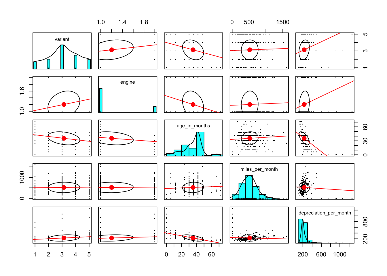
We see that a higher value of age_in_months is associated with a lower value of depreciation_per_month. That feels right, as a vehicle would be expected to lose value more quickly when it was newer. Surprisingly, we do not see that a higher value of miles_per_month is associated with a higher value of depreciation_per_month.

The plot of depreciation_per_month by variant suggests that there might be a high level of association between variant and depreciation_per_month but the fact that variant has only a small number of discrete values and the assumptions about variables being normally distributed mean that we should not put too much weight on the shape of the correlation ellipse for those two variables.

But it might be interesting to view the smoothed distribution of values of depreciation_per_month for each of the variants.

library(ggridges)

cars |> ggplot(
  aes(x = depreciation_per_month, y = variant, fill = variant, color = variant)
) + geom_density_ridges(alpha = 0.5, show.legend = FALSE)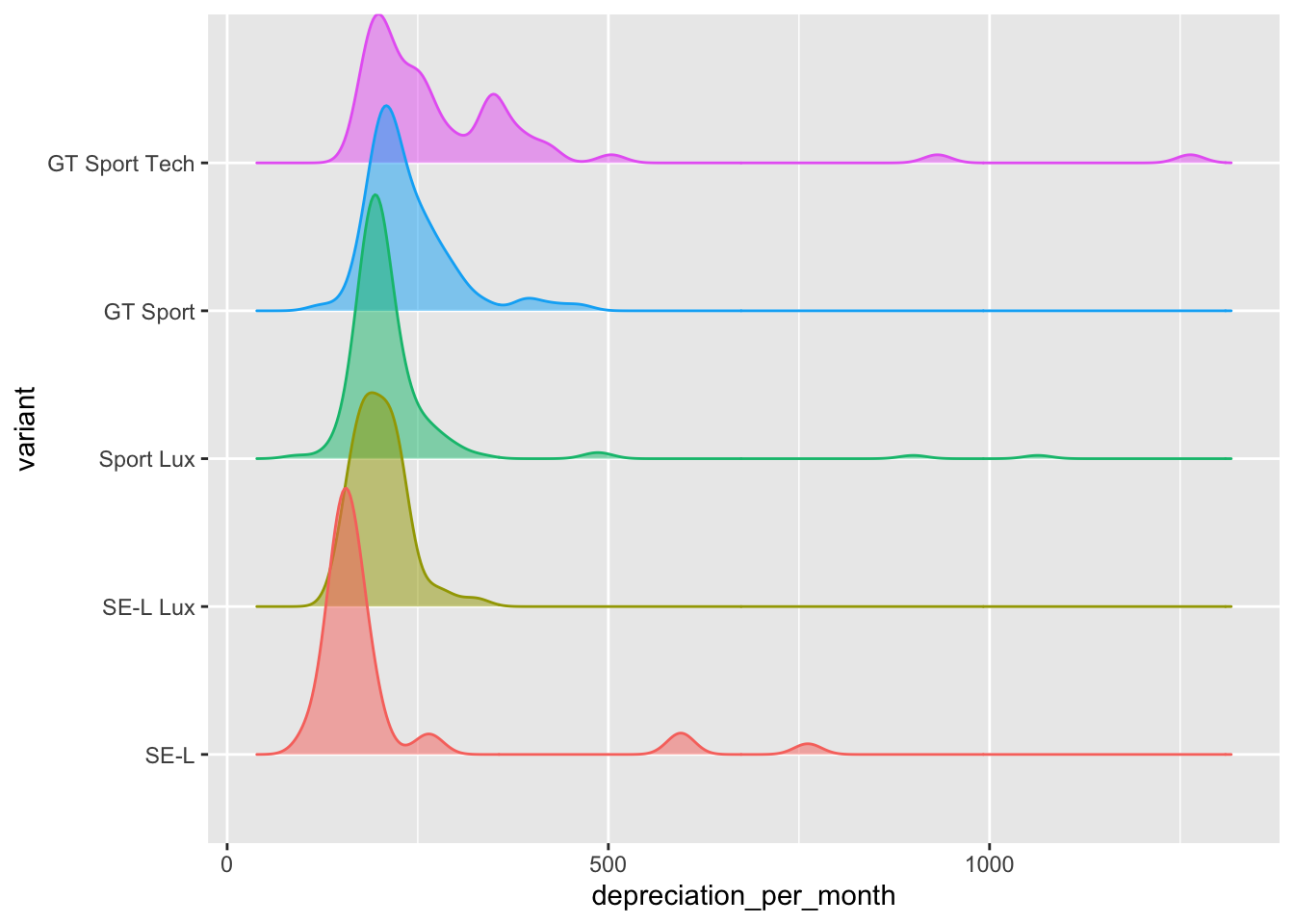

It is noticeable how much narrower the range of depreciation per month is for the cheapest model - the SE-L variant. This is seen even more clearly with a box and whisker plot.

ggplot(
    data = cars,
    mapping = aes(x = depreciation_per_month, y = variant)
) + geom_boxplot(notch = T)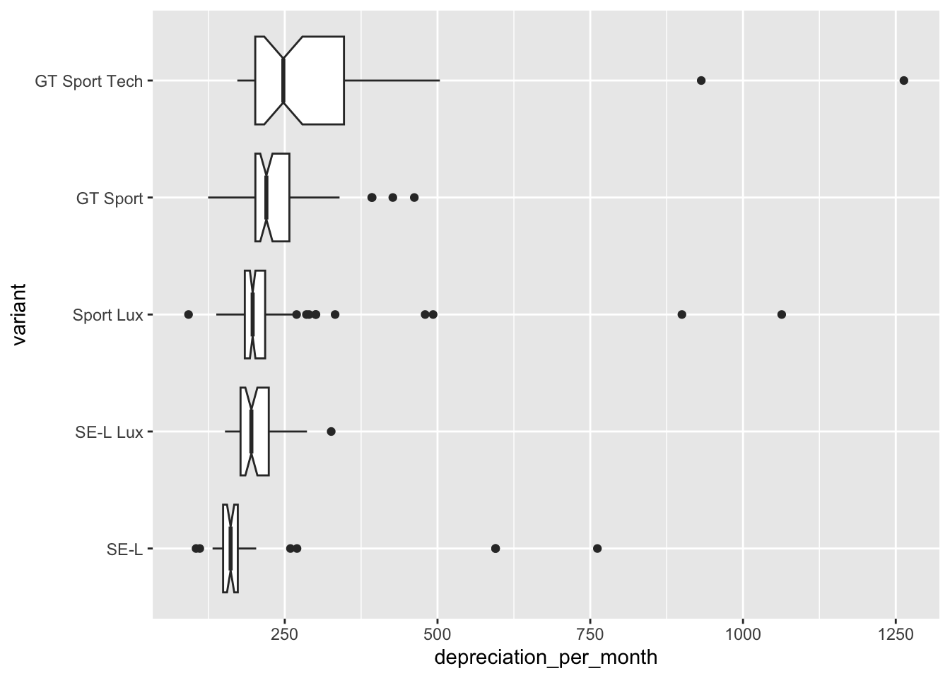

In this plot we have requested a notch on each plot. If the notches on two plots do not overlap then we can assume, with 95% confidence, that the medians are different. So between our variants the median depreciation_per_month is significantly different for all but the SE-L and SE-L Lux variants.

It doesn’t seem too surprising that there would be some vehicles with high levels of depreciation but the low levels are worth examining.

cars |> 
  arrange(depreciation_per_month) |>
  select(model, variant, age_in_months, miles, price, price_new,
    dpm = depreciation_per_month) |>
  head(5)

# A tibble: 5 × 7
  model   variant   age_in_months miles price price_new   dpm
  <fct>   <fct>             <dbl> <dbl> <dbl>     <dbl> <dbl>
1 Mazda 3 Sport Lux            36 19809 24078     27685  92.5
2 Mazda 3 SE-L                 42 17288 18567     23285 105. 
3 Mazda 3 SE-L                 36  9531 18961     23285 111. 
4 Mazda 3 GT Sport             42 24397 21779     27385 125. 
5 Mazda 3 SE-L                 72 11520 13400     23285 132.

We can see that these are all vehicles with a low annual mileage.

The Price distribution by variant shows a potential problem with our data - only one variant (SE-L) is represented in the vehicles over the age of 50 months.

ggplot(
    data = cars,
    aes(x = age_in_months, y = price, color = variant)
) + geom_point()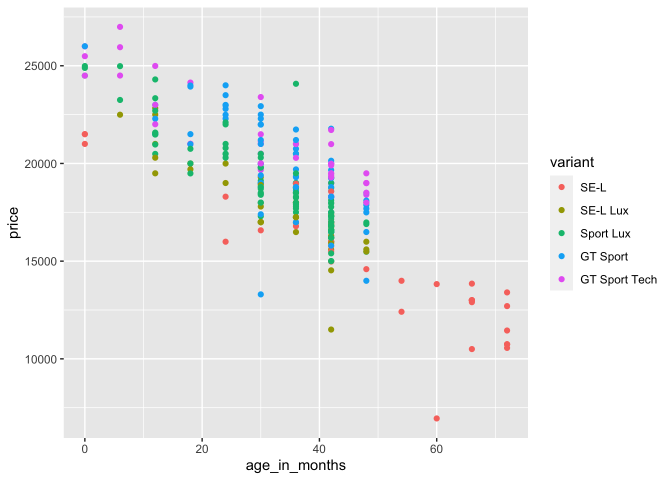

This is seen more clearly when we plot age histograms by variant.

ggplot(
    data = cars,
    aes(x = age_in_months)
) + geom_histogram() + facet_wrap(cars$variant)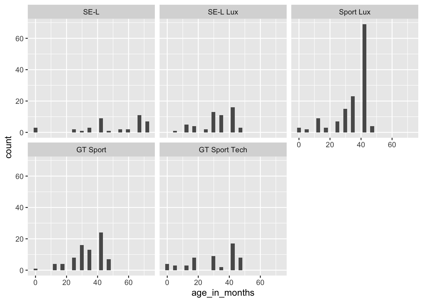

Perhaps that helps to explain why we see a more narrow band of low depreciation_per_month in the SE-L variant.

We can examine the median values of depreciation_per_month by variant in tabular form and this looks to agree nicely with our boxplot above:

cars |>
  select(dpm=depreciation_per_month, variant, engine, drive) |>
  group_by(variant) |>
  summarise(n=n(), median_dpm = median(dpm, na.rm = T)) |>
  arrange(median_dpm) |>
  knitr::kable(digits=0)

variant	n	median_dpm
SE-L	41	161
SE-L Lux	55	195
Sport Lux	135	197
GT Sport	77	220
GT Sport Tech	54	248

By engine across all variants and drives:

cars |>
  select(dpm=depreciation_per_month, variant, engine, drive) |>
  group_by(engine) |>
  summarise(n=n(), median_dpm = median(dpm, na.rm = T)) |>
  arrange(median_dpm) |>
  knitr::kable(digits=0)

engine	n	median_dpm
e-Skyactiv G	289	197
e-Skyactiv X	73	233

So the effect of the more expensive engine looks to be to increase the monthly depreciation by about £36 across all variants and drives.

Or by all combinations of variant and engine (ordered by median depreciation per month).

cars |>
    select(depreciation_per_month, variant, engine) |>
    group_by(variant, engine) |>
    summarise(n=n(), median_dpm = median(depreciation_per_month, na.rm = T)) |>
    arrange(median_dpm) |>
    knitr::kable(digits=0)

variant	engine	n	median_dpm
SE-L	e-Skyactiv G	41	161
SE-L Lux	e-Skyactiv G	50	187
Sport Lux	e-Skyactiv G	109	194
GT Sport	e-Skyactiv G	50	207
SE-L Lux	e-Skyactiv X	5	213
GT Sport Tech	e-Skyactiv G	39	223
Sport Lux	e-Skyactiv X	26	229
GT Sport	e-Skyactiv X	27	233
GT Sport Tech	e-Skyactiv X	15	249

It soon becomes clear that it is difficult to settle on a single method of determining which variables are most explanatory in understanding monthly depreciation. And also, exactly what the numerical effect of the choice of a particular variant or engine might be on monthly depreciation. We have conveniently ignored the effect of the age of the vehicle or the number of miles it has been driven and we know that these are likely to have a big effect.

In the next notebook we will look to model the effect of all of these variables on monthly depreciation.

Next: Mazda 3 Price Data - Modelling