Drawdown: A Go tool to Model Pension Drawdown

Drawdown is a Go tool to model retirement pension drawdown strategies and the influence of external factors on their duration, expected remainder (if any), and the amount lost to taxes.

Pension Drawdown

Author

John Bates

Published

November 21, 2024

Drawdown is a Go command line program that runs an iteration of a pension drawdown strategy to discover how it will unfold over time given a set of sources (pensions, investments, savings accounts) and growth rates (assumed rates of savings and investment growth and inflation) and a period of years over which drawdown will take place. The output of the program shows the balance remaining, the amount withdrawn, and the amount of tax paid at the end of each of the years.

When run with the “-s” command line flag the program will, instead, run the same strategy over each combination of several values of the growth rates to see the impact on the final balance, the amount withdrawn and the amount of tax paid.

The Go code for Drawdown can be found here: https://github.com/Vextasy/Drawdown.

Usage

./drawdown [-s]

The -s flag causes the program to run in summary mode. The output from the program in normal mode will be found in the file drawdown.csv. When run in summary mode the output will be found in the file summary.csv. The output from both of these modes is suitable for use in other programs but, in particular, can be rendered into pivot tables or charts in Excel.

Example Data

The examples shown in this document are based on a simple drawdown strategy that simulates the impact of a withdrawal amount of £35,000 taken annually over a 30 year period for a couple beginning their pension drawdown and who:

Each have a state pension of £10,000 per year with State Pension 1 starting immediately (year 0) and State Pension 2 starting after one year (year 1). The state pension is assumed to increase at the rate of 2.5% per year.
Have £40,000 of savings.
Have £40,000 in an ISA.
Have private pensions: “Pension 1” of £350,000 and “Pension 2” of £150,000.
Have £50,000 in a general investment account (GIA).

In this model, private pensions are assumed to come with a tax-free lump sum of 25% as soon as they enter drawdown - they are effectively split into a taxable drawdown pension of 75% of the original value and a lump sum of 25% of the original value.

When drawdown is run in normal mode (i.e. without the “-s” flag) it uses a fixed set of rate parameters to calculate the situation at the end of each of the 30 years. When run with the “-s” flag it runs the same iterations to completion for every combination of values of the rate parameters.

When run in normal mode the following parameters are used:

const (
    InvestmentGrowthRate     = 3.5  // %
    SavingsGrowthRate        = 3.5  // %
    AnnualInflationRate      = 2.5  // %
    PlatformChargeRate       = 0.25 // The % charge for using a platform as a percentage of the balance.
    TaxBandAnnualPctIncrease = 0.5  // %
)

When run in summary mode the calculation is performed over every combination of the following values (taken at suitable steps):

Investment Growth Rate from 0% to 8%.
Savings Growth Rate from 0% to 8%.
Annual Inflation Rate from 2% to 5%.
Platform Charge Rate from 0.1% to 0.5%.
Tax Band Annual Percentage Increase from 0% to 2%.

These values are built into the program, as are the strategies themselves, but after making a change, a simple recompilation can be performed in less than a second. In this initial version of the program both the parameters and the strategies are altered by editing the Go code. A later version might move the rate parameters to a textual format file and allow the choice from a number of fixed strategies.

Examples of Output - Normal Mode

Actual output of the program takes the form of a CSV file. Different formats are generated for the normal and summary mode of operations but both are suitable for use in another program, such as Microsoft Excel, for the purposes of analysis and visualisation.

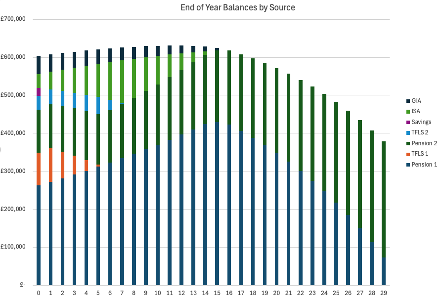
Figure 1 - End of Year Balances by Source

Figure 1 displays an Excel stacked bar-chart that shows, for each of the 30 years for which the iterations were run, the total balance of funds remaining broken down by each source. You can see that the tax-free lump sums (TFLS) shown in orange and blue are exhausted by years 6 and 8 respectively. Also noticeable, is that the ISA balance grows in size up until about year 7, after which is decreases each year until it is used by by year 14. After year 14 the balance is contained wholly within the two pension funds (and also by a couple of state pensions that are not shown in this chart because we don’t consider them to have a balance).

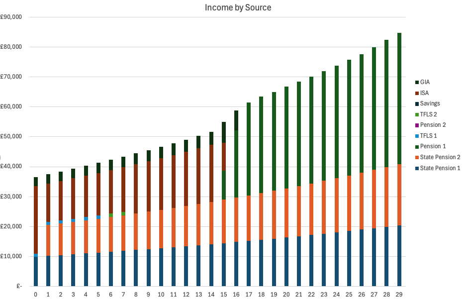
Figure 2 shows the income drawn from the sources each year as a stacked bar-chart with colours being used to identify the size of the contribution from each source. You can see that from year 16 onwards all of the income is coming from the combination of the two state pensions and pension 1. We can also see how a contribution from State Pension 2 didn’t occur until year 1 (because our strategy contains that information) and that because of that a larger amount was drawn from the ISA in year 0.

If you are wondering why the ISA, given that it is used to provide income through to year 15, continues to increase in size, it is because our strategy contains an action that transfers the maximum amount allowed each year from the savings account and the tax free lump sums into the ISA so that it can earn interest over the course of the year in a tax efficient way.

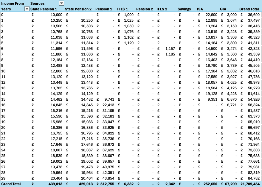
Figure 3 shows a different view of the same information. This time in Pivot Table format you can see, for each of the 30 years, the amount drawn from each source to arrive at the desired annual total figure. The annual total required is calculated from an inflation adjusted annual amount which in this example was set at £35,000 per year. The reason why the total at the end of year 0 is greater than our chosen initial amount is that it is increased to include platform costs for hosting the drawdown pensions and investment and savings accounts. It will also, in later years, be increased by any amount of tax that is incurred when drawing sums from the non-tax-free instruments.

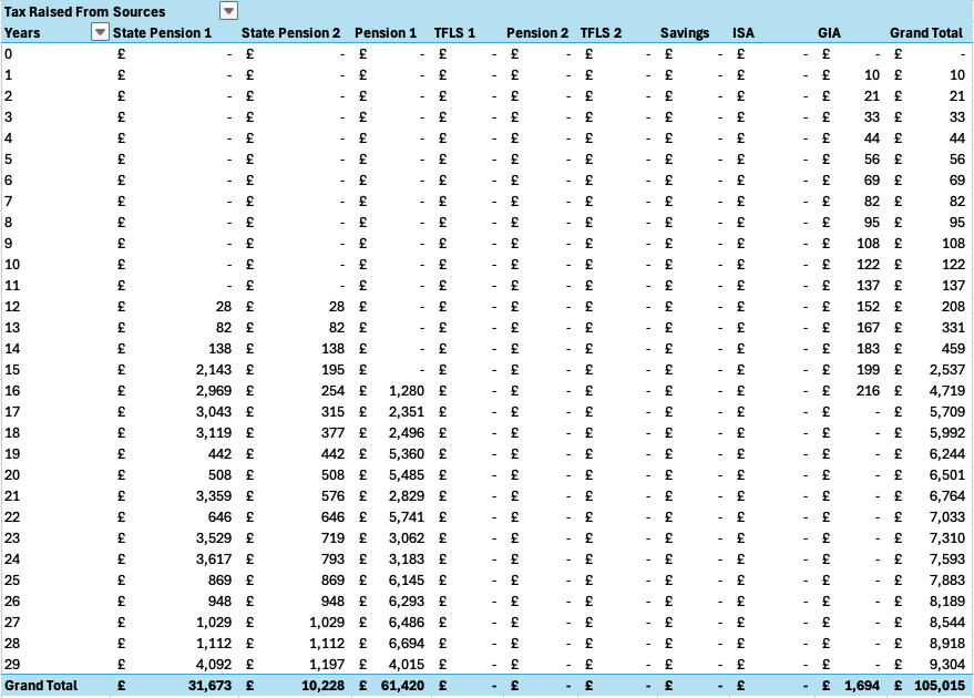
Figure 4 - Tax Raised from each Source Pivot Table

Figure 4 shows that very little tax needs to be paid for the first 15 years because we are mostly drawing income from tax-free sources or, as in the case of the GIA (general investment account), we are keeping our annual withdrawals below the appropriate capital gains tax allowance

Normal Mode Output - Drawdown.csv

The examples above are all built using the normal mode output found in drawdown.csv which looks like this (years 2 to 28 are omitted):

Year,Source,Amount,Tax,Tax Raised,Balance
0,"State Pension 1",10000,0,0,0
0,"State Pension 2",0,0,0,0
0,"Pension 1",0,0,0,262500
0,"TFLS 1",1000,0,0,86500
0,"Pension 2",0,0,0,112500
0,"TFLS 2",0,0,0,37500
0,"Savings",0,0,0,20000
0,"ISA",22600,0,0,37400
0,"GIA",3000,0,0,47000
1,"State Pension 1",10250,0,0,0
1,"State Pension 2",10250,0,0,0
1,"Pension 1",0,0,0,271687
1,"TFLS 1",1025,0,0,88502
1,"Pension 2",0,0,0,116437
1,"TFLS 2",0,0,0,38812
1,"Savings",0,0,0,200
1,"ISA",12898,10,0,46311
1,"GIA",3074,0,10,45570
...
29,"State Pension 1",20464,0,4092,0
29,"State Pension 2",20464,0,1197,0
29,"Pension 1",43854,9304,4015,73198
29,"TFLS 1",0,0,0,0
29,"Pension 2",0,0,0,305066
29,"TFLS 2",0,0,0,0
29,"Savings",0,0,0,0
29,"ISA",0,0,0,0
29,"GIA",0,0,0,0

Each row gives the end-of-year state for a given year and source:

The Amount column is the amount of money that was drawn from that source (including any tax) in the given year.
The Tax column is the amount of tax that was paid from this source in the given year.
The Tax Raised column is the amount of tax incurred as a result of drawing from this source in the given year.
The Balance column is the amount remaining in the source at the end of the given year.

State pensions are assumed to have infinite balance but we return a value of zero for want of a better representation.

You can see from the year 29 rows above that at the end of the 30 year period we are left with a non-zero balance in both of the private pensions as well as still having the two state pensions. We can infer from this that this particular drawdown strategy has preserved the pension pots at the expense of the savings and ISA funds. An alternative strategy might be to drawdown from the pensions first, leaving the tax-free sources until later. This tool allows us to compare the outcome from such different strategies.

Summary Mode Output - Summary.csv

When we run the drawdown program with the “-s” flag we generate a summary output CSV file. In the summary output each row represents a complete iteration of the strategy over the given period of years (in this example 30 years). For each combination of the input rates we obtain values for each of the four output measures of interest.

Investment Growth Rate,Savings Growth Rate,Annual Inflation Rate,Platform Charge Rate,Tax Band Annual Percentage Increase,Total Withdrawn,Tax Paid,Final Balance,Final Year
igr_0.00, sgr_0.00, air_2.00, pcr_0.10, tbi_0.00, 1457098, 81846, 0, 28
igr_0.00, sgr_0.00, air_2.00, pcr_0.10, tbi_0.50, 1498026, 73899, 0, 29
igr_0.00, sgr_0.00, air_2.00, pcr_0.10, tbi_1.00, 1498026, 69204, 0, 29
igr_0.00, sgr_0.00, air_2.00, pcr_0.10, tbi_2.00, 1498026, 56253, 0, 29
igr_0.00, sgr_0.00, air_2.00, pcr_0.25, tbi_0.00, 1457098, 78323, 0, 28
igr_0.00, sgr_0.00, air_2.00, pcr_0.25, tbi_0.50, 1457098, 76125, 0, 28
igr_0.00, sgr_0.00, air_2.00, pcr_0.25, tbi_1.00, 1457098, 66809, 0, 28
igr_0.00, sgr_0.00, air_2.00, pcr_0.25, tbi_2.00, 1498026, 55659, 0, 29
...

The example above shows the first few rows from our summary output file. Each row represents the end result of an iteration over 30 years and gives the following final values:

The Total Withdrawn column is the sum of the amount withdrawn from all of the sources over the iteration (including tax).
The Tax Paid column is the sum of the amount of tax paid from all of the sources over the iteration.
The Final Balance column is the sum of the balance remaining across all of the sources at the end of the iteration.
The Final Year column is the year in which the sources were unable to supply the required needs, or the intended final year of the iteration (if a non-zero balance remains).

These values are given for an iteration for each of several values of input rates:

The Investment Growth Rate column contains the percentage rate at which non-savings investments are assumed to grow each year.
The Savings Growth Rate column contains the percentage rate at which savings investments are assumed to grow each year.
The Annual Inflation Rate column contains the rate at which the needed annual income is increased each year.
The Platform Charge Rate column contains the percentage of the total balance of a source that is charged in fees by the platform each year.
The Tax Band Annual Percentage Increase column contains the percentage rate at which the tax band rates are assumed to be increased each year.

The summary mode output file summary.csv can be easily used by analysis programs, such as Microsoft Excel, to present this data in a useful format.

Examples of Output - Summary Mode

We can import the summary mode data into Excel and visualise it using a combination of pivot tables and charts.

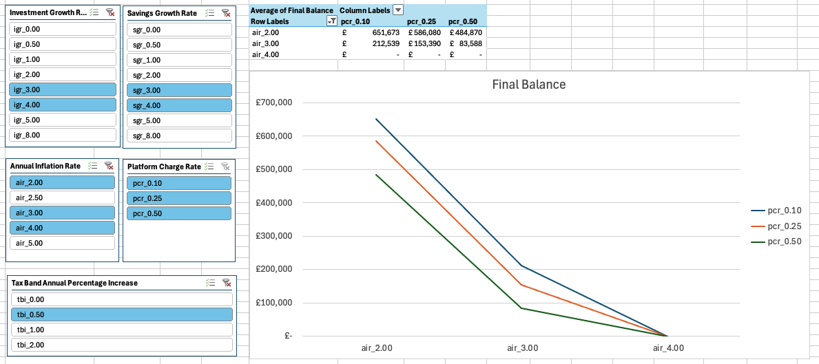
Figure 5 - Final Balance by Platform Charge and Inflation Rate

Figure 5 shows the effect on the final balance of different values of platform charge rate and annual inflation rate. By choosing to display the average final balance figure we can use slicers to select one or more values of each of the other rates and we obtain the average final balance over them. In this example we have averaged over investment and savings growth rates of 3% and 4%, and have fixed the tax band annual percentage increase at 0.5%. We can see from both the pivot table and the chart that with this strategy, its starting balances, annual withdrawal amount and our selected growth rates, the final balance is very dependent on the annual inflation rate. In particular, an annual inflation rate over the retirement period of 4% or higher will mean that we run out of funds before the 30 year period ends.

Another observation is that the level of charges levied by the platform also has a big impact on the final balance. Typically, unless we run out of funds, this is of the order of £150,000.

We can take a closer look at how long our sources will last under different input rates.

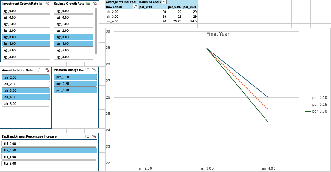
Figure 6 - Final Year by Platform Charge and Inflation Rate

Figure 6 shows that an annual inflation rate of 4% will result in our funds lasting somewhere between 24 and 26 years depending upon the platform charge rate (all other rates being as defined by the sliders).

There are a number of views of the data that can be obtained and which are all useful in understanding how a particular drawdown strategy will unfold given its input rates and starting balances.

The Drawdown Strategy

The elements that define a drawdown strategy are held in a DrawScenario struct.

type DrawScenario struct {
    Sources                  []*Source
    DrawSequence             []*Source
    TaxPaymentSequence       []*Source
    TaxAccounts              map[*Source]*TaxAccount
    TaxRegimes               []*TaxRegime
    Actions                  []func(year int, need int64, s *DrawScenario)
    InflationLinkedVariables []*int64
    Rates                    DrawRates
}

Sources

The Sources field contains a slice of the full set of Sources available to the strategy.

// Source represents something from which income can be drawn.
// This might be a savings account, an investment account, or a pension, for example.
type Source struct {
    Name           string
    balance        int64                             // The amount of money currently in the source.
    year           int                               // The current year (origin zero) - decisions might be based on this.
    startYear      func(year int)                    // Called at the beginning of each year typically to set the opening balance (year origin is zero).
    endYear        func(year int)                    // Called at the end of each year.
    makeWithdrawal func(amount int64) []SourceAmount // nil, else it returns the amount withdrawn from the source.
}

// Type SourceAmount represents an amount of money associated with a given source.
type SourceAmount struct {
    Source *Source
    Amount int64
}

In each year of the iteration, a needed amount is drawn from the sources in the order given by the DrawSequence field. Mechanisms exist to specify that a limit should be put on the amount drawn from a source, or that the amount drawn should be split between two sources, or drawn from a pool of sources in sequence. A source can also appear multiple times in the draw sequence - usually initially with some limit and then later as a source of last resort (when all earlier sources have been exhausted).

The makeWithdrawal function of Source returns a slice of SourceAmount structs. This allows synthetic sources to split withdrawals between a number of real sources.

The Draw Sequence

The draw sequence is the order in which money is withdrawn from the sources to satisfy the calculated amount of money needed each year. It might look something like this:

drawSequence := []*drawdown.Source{
        is_state_pension_1,
        is_state_pension_2,
        drawdown.Seq(&capitalGainsTaxAllowance, is_gia),
        drawdown.Seq(&v1000, is_pension_1_tfls, is_savings, is_pension_2_tfls),
        is_isa,
        is_pension_1_tfls,
        is_pension_2_tfls,
        is_pension_1,
        is_pension_2,
        is_savings,
        is_gia,
    }

In the example above, money is being taken from the sources in the following order:

state pensions first,
an inflation-adjusted tax-free amount from the general investment account,
an inflation-adjusted £1,000 from the tax-free lump sums and savings account,
the ISA,
the tax-free lump sums,
the private pensions,
the savings account,
the general investment account.

Outstanding amounts are withdrawn in that order until the needed quantity has been satisfied. By altering this sequence you can choose to exhaust pensions first, leaving saving and tax-free lump sums, or vice versa, or some other strategy.

Tax

Tax is paid at the end of each year by examining the amount drawn from each source and calculating the tax due on it. The tax is paid by visiting, in order, each of the sources in the TaxPaymentSequence field and making withdrawals from them until the tax amount is paid. If the tax payment sequence contains a taxable source then more tax may be incurred in drawing funds from it, in which case the unpaid tax is added to the needed amount for the following year.

// A TaxAccount records the amount of a money on which tax has already been calculated.
// and also the calculated total amount of tax due on that amount.
type TaxAccount struct {
    Name        string
    regime      TaxRegime
    taxedamount int64 // The amount of money on which tax has already been calculated.
    tax         int64 // The total amount of tax that has been calculated to be due on that amount.
}

The taxed amount and the tax due values are reset in a tax account at the start of each year.

taxAccounts := map[*drawdown.Source]*drawdown.TaxAccount{
    is_state_pension_1: incomeTaxAccount1,
    is_state_pension_2: incomeTaxAccount2,
    is_pension_1:       incomeTaxAccount1,
    is_pension_2:       incomeTaxAccount2,
    is_gia:             capitalGainsTaxAccount,
}

A TaxAccount may be shared by more than one source. For example, all sources which are subject to income tax. At the end of each year, the set of source withdrawals are examined to calculate the tax due in each of the tax accounts.

// TaxRegime describes the rates of tax that are charged on increasing amounts.
// Commonly the first RateBound in the slice might represents a tax-free allowance (i.e. its rate is zero).
type TaxRegime struct {
    Rates []RateBound
}

// RateBound contains a rate and an upper bound on the amount for which the rate applies.
// A slice of RateBound is used to describe a tax regime.
// In such a slice, subsequent upper values must be strictly increasing.
// Rates are represented as a decimal percentage. For example, 10.1 for 10.1%.
type RateBound struct {
    upper int64
    rate  float64
}

A TaxRegime defines the ranges and rates that are associated with a TaxAccount. For example, the following might define an income tax regime:

incomeTaxRegime := drawdown.NewTaxRegime([]drawdown.RateBound{
        drawdown.NewRateBound(12540, 0.0),
        drawdown.NewRateBound(50270, 20.0),
        drawdown.NewRateBound(125140, 40.0),
        drawdown.NewRateBound(drawdown.HighUpperBound, 45.0),
    })

In this regime the first £12,540 of income would be tax free, the next £37,730 (= £50,270 - £12,540) would be taxed at 20%, the next £74,870 (= £125,140 - £50,270) would be taxed at 40%, and any amount above above that would be taxed at the 45% rate.

Actions

Actions are performed at the start of the year after the sources and tax accounts have been initialised and before any withdrawals are made.

actions := []func(year int, need int64, s *drawdown.DrawScenario){
    func(year int, need int64, s *drawdown.DrawScenario) {
        //fmt.Println("year", year, "need", need)
    },
    func(year int, need int64, s *drawdown.DrawScenario) {
        // Every year make the maximum annual ISA contribution from the savings accounts.
        drawdown.Transfer(&annualMaximumIsaContribution, is_isa, is_savings, is_pension_1_tfls, is_pension_2_tfls)
    },
}

An action is a function that is called with three arguments: the year (starting at 0), the amount of money that needs to be withdrawn from the sources in the year (this includes an inflation adjusted increment from the previous year and any unpaid tax from the previous year), and the information in the DrawScenario.

In the example code above an action has been created as a convenient place to include debugging information and also to invoke a function to transfer an amount of money into an ISA account from a savings account, or if no saving are left, from one of the tax-free lump sum accounts.

Inflation-linked Variables

The DrawScenario InflationLinkedVariables slice contains pointers to a number of variables whose value is automatically incremented at the end of each year by the rate of inflation. In the example actions above the annualMaximumIsaContribution is such an inflation-linked variable.

// Inflation linked variables
incomeTaxAllowance := incomeTaxRegime.TaxFreeAllowance()
capitalGainsTaxAllowance := capitalGainsTaxRegime.TaxFreeAllowance()
annualMaximumIsaContribution := int64(20000)
v1000 := int64(1000)

allInflationLinkedVariables := []*int64{
    &annualMaximumIsaContribution,
    &incomeTaxAllowance,
    &capitalGainsTaxAllowance,
    &v1000,
}

You can see from the code above how we maintain our estimate of the likely value of the maximum ISA contribution that can be made each year by increasing its value in line with inflation. Similarly, in the example, v1000 is an inflation linked amount that is equivalent to £1,000 in year 0.

Draw Rates

The DrawRates are those input rates that determine how investments and savings are expected to grow, what the expected annual inflation rate and the annual platform charge are and how quickly to increase the TaxRegime tax bands.

type DrawRates struct {
    InvestmentGrowthRate     float64
    SavingsGrowthRate        float64
    AnnualInflationRate      float64
    PlatformChargeRate       float64
    TaxBandAnnualPctIncrease float64
}

Investment account and savings accounts are initialised using the investment and savings growth rates:

    is_savings := drawdown.NewSavingsAccount("Savings", SavingsInitialBalance, &s.Rates.SavingsGrowthRate)
    is_isa := drawdown.NewInvestmentAccount("ISA", IsaInitialBalance, &s.Rates.InvestmentGrowthRate)

    is_pension_1 := drawdown.NewInvestmentAccount("Pension 1", 0.75*Pension1InitialBalance, &s.Rates.InvestmentGrowthRate)
    is_pension_1_tfls := drawdown.NewSavingsAccount("TFLS 1", 0.25*Pension1InitialBalance, &s.Rates.SavingsGrowthRate)

At the start of the year the amount of money needed is scaled up from the initial year 0 amount by the annual inflation rate and at the end of the year the inflation linked variable are also scaled in the same way.

At the start of the year the platform charge is calculated by adding up the total balance from all of the sources and multiplying it by the PlatformChargeRate. This is then added to the money needed amount in addition to any unpaid tax left over from the previous year to give an amount that needs to be withdrawn from the sources in the year.

At the end of the year the tax regime upper bounds are scaled up by the TaxBandAnnualPctIncrease percentage.

Summary

There are some obvious limitations to the drawdown model that could be improved upon:

It is almost certainly unreasonable to be able to predict any of the rates with a degree of accuracy over a 30 or 40 year period - especially the rate of inflation.
It would be nice to move the configuration of the drawdown strategy out of code and into a textual format (such as JSON) so that the tool could more readily compare multiple strategies as well as multiple rates.

A partial solution to the first limitation is to use the summary mode to examine the effect of a range of values for a given rate. A mitigating factor for the second limitation is that, assuming you are a Go programmer, it is easy and quick to make a change to the strategy by editing the code.

Nevertheless, the tool can be used to get a feel for how comfortably (or not) your desired annual withdrawal can be satisfied from the set of investments and savings that you have at retirement. And, by making changes to the order of withdrawal, by altering the draw sequence, you can experiment with different strategies.

Source Code

The Go code for Drawdown can be found here: https://github.com/Vextasy/Drawdown.

The strategy used in the examples in this document can be found in the source file scenario/simple.go.